Chapter 3 – Dynamics Errors for Fixed-Step Integration Methods

3.1 Introduction

Error analysis of numerical integration algorithms is traditionally based on the residual error terms in the Taylor series expansion representing the integral. Although such error measures do establish the dependence of the error on both the integration step size and the magnitude of the appropriate higher derivative, they do not lend much insight into the estimation of solution errors when applying a given integration algorithm to a specific problem. Indeed, comprehensive error analysis can only be accomplished when the differential equations being integrated are linear, which is seldom the case in most practical applications.

Fortunately, as we have pointed out in Chapter 1, the nonlinear differential equations can often be linearized about some reference or equilibrium solution, at least for purposes of approximate error analysis. If, in addition, the integration step size is taken to be constant (this is invariably the case in real-time simulation of dynamic systems and can be approximately true over a number of integration steps when a variable-step method is used), then the Z-transform theory introduced in Chapter 2 can be applied. This in turn allows analytic formulas to be developed for the errors in quasi-linear system characteristic roots and the gain and phase errors in the quasi-linear system transfer functions. These specific error measures have already been defined in Chapter 1, Eqs. (1.45), (1.47), (1.49), (1.50), (1.53), (1.54) and (1.55). They will depend on the integration step size as well as the particular integration algorithm, and can be directly related in a meaningful manner to the overall solution accuracy in simulating dynamic systems.

In this Chapter the characteristic root and transfer-function gain and phase errors are developed in convenient asymptotic form for a variety of integration methods. For single-pass (or equivalent single-pass) integration algorithms we will show that the characteristic root errors and transfer-function gain and phase errors can easily be written for any order of linear system based on knowledge of the gain and phase errors of the algorithm in performing simple isolated integration. The frequency-domain methodology developed in this chapter not only allows quantitative comparison of the dynamic performance of various integration methods, but it also points the way to developing improved algorithms in specific applications.

3.2 Error Measures for Euler Integration

We now illustrate the methodology for deriving the error measures defined in Chapter 1 by considering the most simple of all integration methods, Euler or rectangular integration, when applied to the solution of the first-order linear system described by the state equation

(3.1)

This is the example we considered earlier in Chapter 2 to illustrate the Z-transform method. If we use Euler integration to solve Eq. (3.1) numerically, the following difference equation is employed:

(3.2)

3-1

where h is the integration step size and x_n = x(nh), u_n = u(nh) Taking the Z transform of Eq. (3.2), we have

(3.3)

For x₀ = 0 (zero initial condition) we obtain the following formula for the digital system Z transform:

(3.4)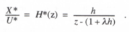

As noted in Eq. (2.22), the pole, z₁ = 1 + λh, of H*(z) is related to the equivalent characteristic root, λ*, by the formula

(3.5)

from which

(3.6)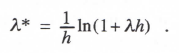

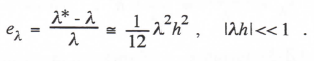
We can derive an asymptotic formula for λ* when |λh| << 1 by letting z = e^λ*h = 1 + λ*h + (λ*h)²/2 + ··· in the denominator of Eq. (3.4). Setting the denominator equal to zero and retaining terms up to h², we obtain

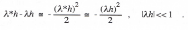
This gives us the following formula for the fractional error in characteristic root:

(3.7)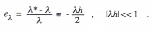

This is just the result we obtained earlier in Eq. (2.24) by expanding the log function of Eq. (3.6) in a power series. Here we have obtained the asymptotic formula for e_λ directly from the denominator of the system Z transform. This is also the method we will use later in this chapter in the case of higher-order integration methods, where it is not possible to derive analytic formulas for the poles of the system Z transform.

Next we derive the asymptotic formula for the fractional error in the digital system transfer function for sinusoidal inputs. From Eq. (2.39) we have

(3.8)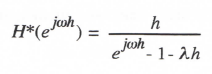

for the digital system transfer function. From Eq. (2.40) the continuous system transfer function for sinusoidal inputs is

(3.9)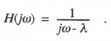

3-2

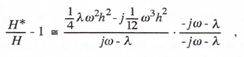
From Eqs. (3.8) and (3.9) we can write the exact formula for H*/H – 1, the fractional error in digital system transfer function. In trigonometric form the formula is given in Eq. (2.41). To derive a simpler asymptotic expression when ωh <<1 , we expand the exponential function in the denominator of Eq. (3.8) in a power series and retain terms of order h². In this way we obtain

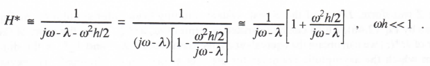
(3.10)

Noting that 1/(jω – λ) = H from Eq. (3.9), we can write the following formula for the fractional error in digital system transfer function:

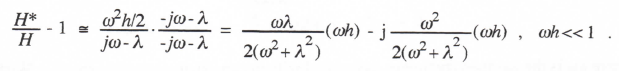
Comparison with Eqs. (1.53) and (1.54) leads directly to the following asymptotic formulas for the transfer function gain and phase errors:

(3.11)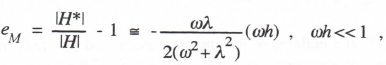

(3.12)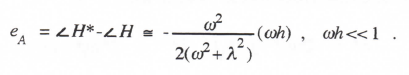

As expected, the transfer function gain and phase errors using Euler integration vary as the first power of the integration step size h.

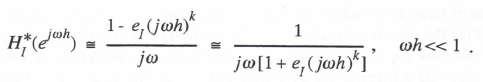
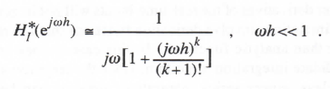
Reference to Eq. (3.1) shows that when λ = 0, the linear first-order system represents a pure integrator. The corresponding Euler integrator transfer function, H_I*, can be written directly in asymptotic form by setting λ = 0 in Eq. (3.10). In this way we obtain

(3.13)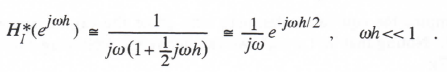

From Eq. (3.13) it is evident that Euler integration behaves approximately as an ideal integrator (transfer function =1/jω) with an additional phase lag of ωh/2, which in turn corresponds to a pure time delay of h/2.

We consider next the case where the characteristic root (eigenvalue) is complex. This will occur in simulating an underdamped second-order linear system, such as the mass-spring-damper system given by Eq. (2.42). In terms of the undamped natural frequency ω_n (= √K/M) and the damping ratio ζ(=C/2√KM) Eq. (2.42) can be rewritten as

(3.14)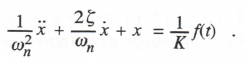

3.3

For the underdamped case, ζ < 1, and the characteristic roots λ₁ and λ₂ are given by

(3.15)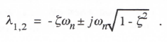

The Z transform, H*(z), of the digital system resulting from Euler simulation of Eq. (3.14), is given by Eq. (2.46), which can be rewritten in terms of ω_n and ζ. From the roots of the denominator of H*(z) we can obtain the equivalent characteristic roots, λ₁* and λ₂*, of the digital system, from which the asymptotic formulas for the root errors can be obtained. However, a simpler procedure is to use Eq. (3.7), as obtained for Euler simulation of the first-order system, but with λ complex. Thus we let λ in Eq. (3.7) be given by

(3.16)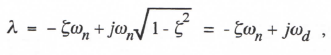

where ω_d is the damped frequency associated with the continuous-system root λ. With Eq. (3.16) for λ, Eq. (3.7) becomes

(3.17)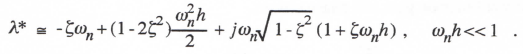

In terms of ω_n* and ζ*, the undamped natural frequency and damping ratio, respectively, of the equivalent digital system characteristic root λ*, we can write λ* as

(3.18)

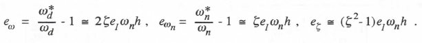
where ω_d* is the damped frequency associated with λ*. Comparison of Eq. (3.17) with (3.16) shows that ζω_nh in Eq. (3.17) represents e_ω, the fractional error in the damped frequency of the digital root. Thus for Euler integration

(3.19)

To compute the equivalent damping ratio ζ* of the digital system root, we must first determine ω_n*. Noting that |λ*| = ω_n*, we can derive the following asymptotic formula for ω_n* from Eq. (3.17):

(3.20)

It follows that eω_n the fractional error in undamped natural frequency of the digital root as defined

previously in Eq. (1.49), is given for Euler integration by

(3.21)

Equating the real part of λ* in Eq. (3.17) to – ζ*ω_n* with ω_n* given by Eq. (3.20), we obtain the following asymptotic formula for the damping ratio error when using Euler integration:

3-4

(3.22)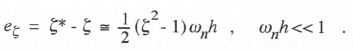

From Eqs. (3.19), (3.21) and (3.22) it is evident that the error parameters associated with complex characteristic roots when using Euler integration all vary as the first power of the integration step size h.

It is interesting to note from Eq. (3.19) that when ζ = 0, there is no error in the frequency of the simulation to order h when using Euler integration. There is, however, a frequency error of order h². On the other hand, Eq. (3.22) shows that for ζ = 0 when using Euler integration, the damping-ratio error eζ – ω_nh/2. Thus the digital system damping ratio ζ* – ω_nh/2 instead of the continuous system damping ratio of ζ = 0. Figure 3.1 shows the solution obtained by Euler integration for the specific case of ω_n = 1 and h = 0.1, which means that ζ* – ω_nh = -0.05. Because of the negative damping ratio, the oscillatory Euler solution grows instead of remaining constant. For the characteristic root pair given by Eq. (3.15) it is apparent that the associated transient x₁ with ζ < 1 for the continuous solution will have the form

(3.23)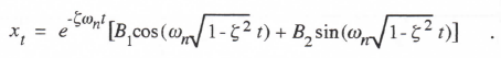

Since the period T of the oscillatory transient is given by 2π/(ω_n√1 – ζ²) , it follows that the ratio of successive peaks in the oscillatory transient, as reflected by the change over one cycle in the exponential amplitude factor e-wig, will be given by

(3.24)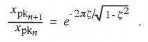

Taking the log of both sides, we obtain

(3.25)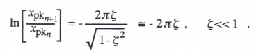

For ζ < < 1 it follows from Eq. (3.25) that ^xpk_n+1 ^xpk_n and therefore | ^xpk_n+1^/xpk_{n-1| << 1.}

Under these conditions we can rewrite Eq. (3.25) as

(3.26)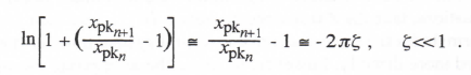

In the Euler simulation in Figure 3.1, we have seen above that ζ* -0.05 for ω_nh = 0.1, according to Eq. (3.22). Letting ζ* = ζ = -0.05 in Eq. (3.26), we find that ^xpk_n+1/ ^xpk_n – 1 0.1π = 0.314. Thus we expect a fractional increase of approximately 0.314 each cycle of the oscillatory transient when the damping ratio is -0.05. This is indeed confirmed in the solution shown in the figure. Clearly Euler integration is not a very efficient algorithm for simulating an undamped second-order system.

We next consider the transfer function errors when Euler integration is used to simulate the second-order linear differential equation given by

3-5

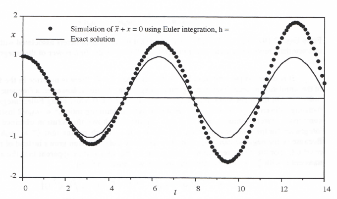
Figure 3.1. Undamped second-order system simulation using Euler integration.

1

(3.27)

The transfer function of the continuous system for sinusoidal inputs becomes

(3.28)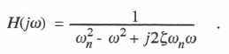

We could, of course, use the same procedure we employed earlier in analyzing the transfer function errors in the case of Euler integration of the first-order linear system, namely, write the difference equations, take the Z transform to obtain H*(z), and then from H*(e^jwh) determine the asymptotic formula for the fractional error in digital system transfer function. The error formulas can be obtained more directly, however, by using the asymptotic representation of Eq. (3.13) for the transfer function of the Euler integrator. Thus we replace jω in Eq. (3.28) by jω (1 + jωh/2). In this way we obtain

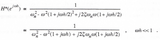(3.29)

From Eq. (3.29) the following asymptotic formula for the fractional error in transfer function follows directly:

3-6

(3.30)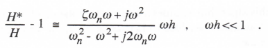

After rationalization to obtain the real and imaginary parts of H*/H – 1, the following formulas are obtained for the fractional error in transfer function gain and the phase error for Euler integration applied to a second-order linear system:

(3.31)

Again we note that the transfer function gain and phase errors for Euler integration, applied here to the simulation of a linear second-order system, are proportional to the first power of the integration step size h.

3.3 Error Measures for Single-pass Integration Algorithms in General

In the previous section we developed characteristic root and sinusoidal transfer function error formulas for Euler integration of first and second-order linear systems. We used procedures in deriving these formulas that can be generalized to any single-pass integration method. By a single-pass method we mean an integration algorithm which requires only one evaluation of each state-variable derivative per overall integration step. Any of the Adams-Bashforth predictor methods, as well as the trapezoidal and other implicit methods introduced in Chapter 1, qualify as single-pass methods. Although the Adams-Moulton predictor-corrector methods of Chapter 1 require two passes per integration step, they still produce asymptotic errors identical to those of the equivalent implicit methods. This is because the local integration truncation error associated with the predictor pass, as described in Section 1.2, is of order k + 1 for a kth-order Adams-Moulton method and will therefore not contribute to the global error of order k for the overall algorithm. On the other hand the Runge-Kutta methods represent multiple-pass algorithms for which the asymptotic errors are not equivalent to those of any single-pass method. This is because the intermediate passes have local truncation errors of order k or less for kth-order Runge-Kutta methods.

With single-pass algorithms all of the asymptotic formulas for the characteristic-root and transfer-function errors can be written directly once the approximate formulas for each individual integrator sinusoidal transfer function are known. Eq. (3.13) represents this formula in the case of Euler integration. As a next example we consider second-order Adams-Bashforth (AB-2) integration. From Eq. (1.12) the AB-2 difference equation for simple integration of the equation dx/dt = f(t) is given by

(3.32)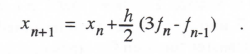

3-7

Based on f_n and f_n-1 this algorithm assumes a linear extrapolation of f(t) from t = nh to (n+1)h. The area under this extrapolation is added to x_n to compute x_n+1. Taking the Z transform of Eq. (3.32) with x₀ = 0, we have

(3.33)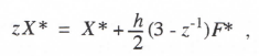

from which the following formula is obtained for the AB-2 integrator Z transform:

(3.34)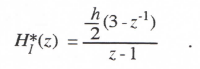

The integrator transfer function for sinusoidal input data sequences is given by H_I*(e^jωh). Thus

(3.35)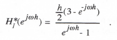

If we represent the exponential terms in Eq. (3.35) by power series and retain terms to order h³, then the following asymptotic formula is obtained for the AB-2 integrator transfer function:

(3.36)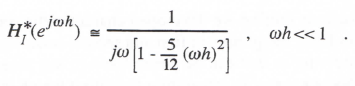

Comparison with the ideal integrator transfer function of 1/jω shows that the AB-2 integrator behaves approximately like an ideal integrator except for a fractional gain error equal to (5/12)(ωh)². To order h² the AB-2 integrator phase error is zero.

We will now show that for any kth-order numerical integration algorithm the asymptotic formula for the integrator transfer function takes the form

(3.37)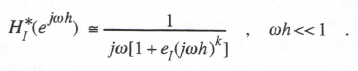

In Section 1.2 we have seen that an appropriate Taylor series expansion for a kth-order integration algorithm can be used to derive the following formula for x_n+1 – x_n:

(3.38)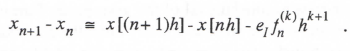

Here x[(n+1)h] and x[nh] represent the exact solution of the continuous integral of f(t) at times (n+1)h and nh, respectively, and the term –e_I f h^k+1 represents the local truncation error associated with the integration method of order k, where f is the kth time derivative of f at t = nh. For example, Eq. (1.7) in Section 1.2 shows that k = 1 and e_I = 1/2 for Euler integration; for trapezoidal integration k = 2 and e_I = -1/12, as determined earlier in Eq. (1.10). To develop formulas for the integrator transfer function for sinusoidal inputs we take the Z transform of Eq. (338) and divide by z -1 to obtain

3-8

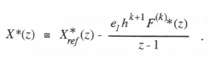
(3.39)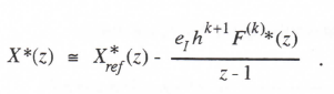

Here X*_ref (z) is the Z transform of the exact solution, x[nh]. Next we consider the case of sinusoidal data sequences by replacing z with e^jωh. We also note that F^(k)*(e^jωh) = (jω)^k F* (e^jωh), i.e., the Fourier transform of the kth derivative of a function is equal to the Fourier transform of the function multiplied by (jω)^k. After dividing the resulting expression by F*, we have

(3.40)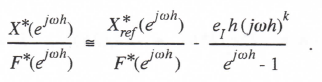

The term X*/F* is simply the sinusoidal transfer function, H_I* (e^jωh), of the numerical integrator. The term X*_ref /F*=1/jω, the transfer function of an ideal integrator. If we now approximate e^jωh -1 by jωh, Eq. (3.40) can be rewritten as

Thus Eq. (3.37) is verified as representative of the general asymptotic form for the transfer function of a numerical integrator of order k. Comparison of Eq. (3.37) with Eq. (3.13) shows that for Euler integration, k = 1and e_I = 1/2. Comparison of Eq. (3.37) with (3.36) shows that for AB-2 integration, K = 2 and e_I = 5/12 . Table 3.1 on page 3-51 of this chapter presents summary formulas for the integrator transfer function error coefficient e_I for predictor, predictor-corrector, power series and implicit integration algorithms up to order K = 4.

For any single-pass integration algorithm it is straightforward to show that the Z transform of the digital system that results when the algorithm is used to simulate a linear system with transfer function H(s) is given by

(3.41)

i.e., the argument s in H(s) is simply replaced by 1/H_I*(z). This is because H_I*(z) is the digital equivalent to 1/s for the continuous system and therefore 1/H_I*(z) is equivalent to s. In the same way, the digital system transfer function for sinusoidal inputs for any single pass integration algorithm used to simulate a continuous system with transfer function H(jω) is given by

(3.42)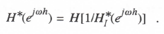

In particular, let H(s) = 1/(s – λ) and H(jω) = 1/(jω – λ). Using Eq. (3.37) to represent H_I*, the general asymptotic form of the integrator transfer function, we obtain the following formula for the digital system transfer function for sinusoidal inputs:

(3.43)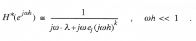

3.9

Replacing jω with λ* and solving for 1/H*, we obtain

(3.44)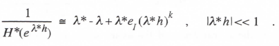

Setting the right side of Eq. (3.44) equal to zero and solving for λ* determines the value of λ* which makes the denominator of H*(e^λ*h) vanish, i.e., the equivalent characteristic root of the digital system. Thus

and

(3.45)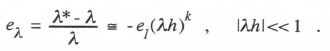

Eq. (3.45) represents an asymptotic formula for the fractional error in characteristic root for any single-pass or equivalent single-pass algorithm, where e_I is the integrator transfer-function error coefficient for the specific algorithm. We have already seen for Euler integration that k = 1 and e_I = 1/2. In this case Eq. (3.48) yields e_λ – λh/2, which is precisely the result we derived earlier in Eq. (3.7). For AB-2 integration we found that k = 2 and e_I = 5/12. From Eq. (3.48) it follows that – (5/12)(λh)² is the asymptotic formula for e_λ , the fractional error in characteristic root when using the AB-2 algorithm.

It should be noted that Eq. (3.45) is not valid for multiple-pass integration algorithms where the intermediate passes used to obtain the states for the final pass are of order less than k. Thus Eq. (3.48) is not valid for the Runge-Kutta methods. On the other hand it is valid for the two-pass Adams-Moulton algorithms introduced in Chapter 1.

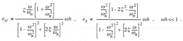
From Eq. (3.43) it is easy to obtain the asymptotic formula for the fractional error in sinusoidal transfer function. If we factor jω – λ from the denominator and note that 1/(jω – λ) = H(jω) , we can obtain the following formula:

(3.46)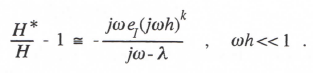

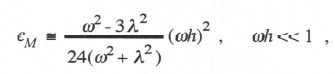
To obtain the separate real and imaginary parts of H*/H-1 we must rationalize the right side of Eq. (3.46). The result will depend on whether the order k of the integration algorithm is odd or even. We obtain the following formulas for e_M, the fractional error in transfer-function gain (i.e., the real part of H*/H-1), and e_A, the transfer function phase error (i.e., the imaginary part of H*/H-1) for k odd:

(3.47)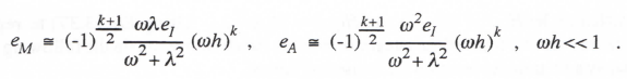

On the other hand for k even we have

3-10

(3.48)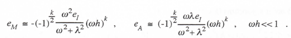

For k = 1 and, e_I = 1/2, e_M and e_A, as given by Eq. (3.47) agree with the asymptotic formulas derived earlier for Euler integration in Eqs. (3.11) and (3.12).

Thus far in this section we have developed general formulas for the characteristic root and transfer function errors when using single-pass integration methods to simulate first-order linear systems. We now derive general formulas for these same error measures when simulating second-order linear systems with complex roots. From Eq. (3.45) the formula for the digital system characteristic root λ* when using a kth-order integration algorithm with error coefficient e_I is given by

(3.49)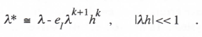

With λ expressed in terms of ω_n and ζ as in Eq. (3.16), Eq. (3.49) can be rewritten for any order k of integration method. To obtain the characteristic-root error coefficients in general for each k we follow the same procedure used to obtain Eqs. (3.19), (3.21), and (3.22) for Euler integration. Thus we note that

(3.50)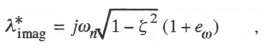

from which the approximate formula for e_ω the fractional error in root frequency , can be obtained. Next we note that

(3.51)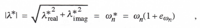

from which the approximate formulas for both ω_n*, the undamped natural frequency of the digital root, and eω_n, the fractional error in the undamped natural frequency, can be written. Finally, we note that

(3.52)

from which the approximate formula for e_ζ, the damping ratio error, can be written. In this way the following asymptotic formulas for e_ω , eω_n and e_ζ. are obtained for k = 1, 2, 3, and 4:

First-order algorithms (k = 1), ω_nh << 1

(3.53)

Second-order algorithms (k – 2), ω_nh << 1,

(3.54)

3-11

Third-order algorithms (k = 3), ω_nh << 1,

(3.55)

Fourth-order algorithms (k = 4), ω_nh << 1,

(3.56)

We next consider the derivation of the approximate formulas for sinusoidal transfer function gain and phase errors when single-pass integration algorithms are used to simulate a second-order linear system. In Section 3.2 we derived these formulas for Euler integration by substituting the asymptotic representation of the Euler integrator transfer function into the second-order continuous-system transfer function H(jω). We use the same procedure here by employing Eqs. (3.37) and (3.42), where H(jω) is given by Eq. (3.28). Thus

(3.57)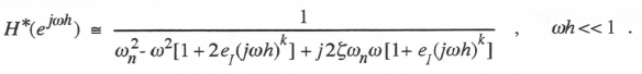

If we factor out ω_n² – ω² + j2ζω_nω from the denominator and set the factor equal to 1/H(jω), we can obtain the following formula for the approximate fractional error in digital system transfer function:

(3.58)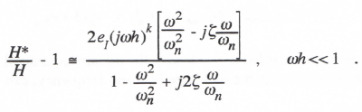

To obtain the separate real and imaginary parts of H*/H – 1 we must rationalize the right side of Eq. (3.58). The result will depend on whether the order k of the integration algorithm is odd or even. The following formulas are obtained for the fractional gain error e_M and the phase error e_A of the transfer function when k is odd:

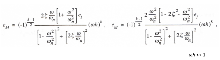
(3.59)

For even k the formulas are

3-12

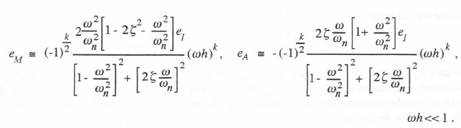
(3.60)

Thus far in this section we have derived formulas for transfer-function gain and phase errors for single-pass (or equivalent single-pass) integration algorithms in the simulation of first and second-order linear subsystems. It turns out that the transfer function gain and phase errors in simulating any order of linear system are equal approximately to the sum of the gain and phase errors of the individual subsystems which, when connected in series, represent the overall system. In particular, let the overall transfer function of the continuous linear system be given by

(3.61)

Here λ₁, λ₂, … , λ_n represent the n poles of H(s), i.e., the characteristic roots of the linear
system, and λ_n+1, λ_n+2, … , λ_n+m represent the m zeros of H(s), where m ≤ n. From Eq. (3.42) we can write the following formula for the digital system transfer function for sinusoidal inputs:

(3.62)

where H_I* is the sinusoidal transfer function of the integrator used in the digital simulation of the system.

Consider next the factor (1/H_I* – λ_q) in the denominator of Eq. (3.62). Let H_q* represent the reciprocal of this factor, i.e.,

(3.63)

If we denote eM_q and eA_q, as the real and imaginary parts of the fractional error in the digital transfer function represented by H_q*, i.e., H_q* / H_q – 1 i.e., as defined in Eq. (1.51), then H_q* can be represented as

(3.64)

Here H_q = (jω – λ_q)^-1, the sinusoidal transfer function for the factor (s – λ_q)^-1 in Eq. (3.61). Next, consider the factor (1/H_I* – λ_n+q) in the numerator of Eq. (3.62). Let H*_n+q be the transfer function representing the reciprocal of this factor, i.e.,

(3.65)

3.13

Then we can write

(3.66)

where eM_n+q and eA_n+q are the real and imaginary parts of the fractional error in the digital transfer function represented by H*_n+q, i.e., H*_n+q/H_n+q – 1 and H_n+q = (jω – λ_n+q)^-1. In terms of the individual transfer-function factors defined above, the overall digital system transfer function of Eq. (3.62) can be written as

(3.67)

Substituting Eqs. (3.64) and (3.66) for the individual transfer-function factors on the right side of Eq. (3.67) and neglecting terms above first order in the errors eM_q and eA_q, we obtain the following formula for the fractional error in the overall digital system transfer function:

(3.68)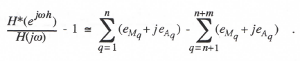

Comparison with Eqs. (1.53) and (1.54) yields the formulas shown below for the fractional error in gain and the phase error, respectively, of the overall digital system transfer function.

(3.69)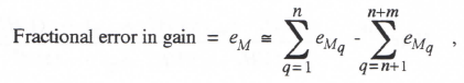

(3.70)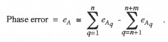

Eqs. (3.69) and (3.70) are completely general and quite useful. They state that the transfer-function gain and phase errors in digital simulation of any order of linear system when using a single-pass (or equivalent single-pass) integration algorithm are equal to the sum of the gain and phase errors, respectively, in simulation of the individual pole and zero factors in the transfer function. For eM_q and eA_q in Eqs. (3.69) and (3.70) we have developed simple asymptotic formulas in terms of the integrator error coefficient, e₁, for factors with real poles or zeros in Eqs. (3.47) and (3.48), and for factors with complex poles or zeros in Eqs. (3.59) and (3.60).

3.4 Adams-Bashforth Predictor Algorithms

In the next several sections we consider a number of well known single pass (or equivalent single-pass) integration methods. For each method we determine the integrator error coefficient e₁ which, along with the order k of the algorithm, allows us to use the formulas developed in the previous section to determine errors in characteristic roots and errors in the gain and phase of the sinusoidal transfer function when simulating any time-invarient linear system.

3-14

First we consider Adams-Bashforth methods up to 4th order. Euler integration could be called AB-1, since it is first-order (k = 1) and is based on a zero-order extrapolation of the state-variable derivative over the integration step h. We have seen that e₁ = 1/2 for Euler integration; this means that the fractional error in characteristic root will be – λh/2, as is evident in Eq. (3.7). It also means that the transfer-function errors will be proportional to ωh/2, as is evident in Eqs. (3.11) and (3.12).

AB-2 integration, represented in Eq. (3.32), is based on the area under a first-order extrapolation from the current and past state-variable derivatives. We have seen that e₁ = 5/12 and k = 2 for AB-2 integration. This means that characteristic root errors will be proportional to (5/12)(λh)² and transfer function errors will be proportional to (5/12)(ωh)².

AB-3 integration, represented in Eq. (1.16), is based on the area under a quadratic extrapolation from the current and past two state-variable derivatives. For integration of the equation dx/dt = u(t), this results in the following difference equation:

(3.71)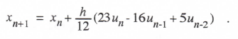

Taking the Z transform and solving for X*/U*, we obtain the AB-3 integrator Z transform. Thus

(3.72)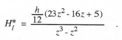

The AB-3 integrator transfer function for sinusoidal inputs is simply H_I*(e^jωh), which takes the following asymptotic form when the exponential functions are replaced by power series with terms retained up to order h⁴:

(3.73)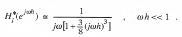

Comparison with Eq. (337) shows that e_I = 3/8 and k = 3 for AB-3 integration.

AB-4 integration, represented by Eq. (1.18), is based on the area under a cubic extrapolation using the current and past three state-variable derivatives. Integration of the equation dx/dt = u(t) leads to the following difference equation:

(3.74)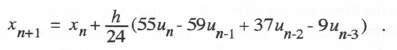

Taking the Z transform and solving for X*/U*, we obtain the AB-4 integrator Z transform. Thus

(3.75)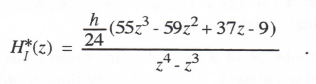

3-15

The AB-4 integrator transfer function for sinusoidal inputs is simply H_I*(e^jωh), which takes the following asymptotic form when the exponential functions are replaced by power series with terms retained up to order h⁵:

(3.76)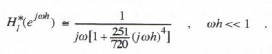

Comparison with Eq. (3.37) shows that e_I = 251/720 and k = 4 for AB-4 integration.

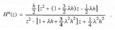
Before considering any additional single-pass methods, let us discuss the extraneous roots which result from the AB predictor methods. Assume we use AB-2, for example, to solve the first-order linear system of Eq. (3.1), which has the transfer function H(s) = 1/(s – λ). According to Eq. (3.41) we can write the Z transform of the resulting digital system by simply replacing s in H(s) with 1/H_I*, where H_I* for AB-2 integration is given by Eq. (3.34). In this way we obtain

(3.77)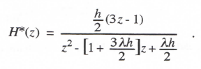

We note that H*(z) has two poles because the denominator is a quadratic in z. One of these poles, z₁, corresponds to an equivalent characteristic root λ* which will almost equal the ideal root λ when |λh| << 1. The second pole, z₂, corresponds to a second characteristic root, which is extraneous. In solving Eq. (3.1) with AB-2 integration, the second root results from the dependence of the state-variable derivative, f = dx/dt = λx + u(t), on the state x. Since the AB-2 algorithm uses f_n-1 as well as f_n, in this case the next state x_n+1 will depend not only on x_n but also x_n-1. Thus both x_n and x_n-1 become states and a second characteristic root is introduced. For small integration step sizes (|λh| << 1) it can be shown that z₂ λh/2 and therefore corresponds to a transient that decays rapidly in comparison to e^λt for λ negative real

.

In Chapter 2, Figure 2.3, we observed that whenever a pole of H*(z) lies outside the unit circle in the z plane, i.e., exceeds unity in magnitude, the corresponding characteristic root λ* will have a positive real part, leading to an unstable transient. When a pole of H*(z) lies on the unit circle, the system is neutrally stable. Thus all the poles of H*(z) must lie inside the unit circle in the z plane for the digital system to be stable. If Eq. (3.1) is to represent a stable continuous system, then λ < 0 for real λ and the dimensionless step size λh is negative. For λh = -1 it is apparent from the denominator of Eq. (3.77) that z = -1 is a pole of H*(z). From Figure 2.3 we see that the corresponding λ* is equal to jπ/h, which represents an undamped oscillation at one-half the integration frame rate1/h. This causes a neutrally stable transient that results from the extraneous root. For any larger integration step size (λh < -1) the extraneous root causes an unstable transient and the solution diverges, even though the first pole, z₁, corresponding to the principal root, represents a stable solution.

For AB-2 simulation of a second-order system there will be two extraneous roots in addition to the two principal roots. The locus of the dimensionless step values λh for which a pole of H*(z) lies on the unit circle can be calculated by setting the denominator of Eq. (3.77) equal to zero with |z| = 1 and solving for λh. In particular, we let z = e^jθ and vary the polar angle θ between

3-16

-π and π. This generates the plot shown for AB-2 in Figure 3.2. Also shown in the figure are plots of the stability boundaries for AB-3 and AB-4 integration. Only the upper half of each stability boundary is shown, since all plots will be symmetric with respect to the real axis. For all characteristic roots λ and step sizes h such that the product λh remains inside the AB-2 boundary shown in the figure, a digital system that uses AB-2 integration will be stable. For λh values lying outside the boundary, the digital system will be unstable. The frequency of oscillation is generally less than one-half the integration frame rate 1/h. The one exception, noted above, is when λh = -1, in which case the digital system exhibits neutral stability at one-half the sample frequency (frame rate), 1/h, when AB-2 integration is used.

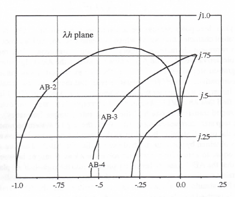
Figure 3.2. Stability boundaries for Adams-Bashforth integration.

Note in Figure 3.2 that the stability boundary for AB-2 integration lies almost directly on the imaginary axis when (λh)_imag <0.3. It follows that if the system being simulated has a root λ on the imaginary axis with a magnitude |λ| < 0.3/h, which corresponds to an undamped transient, the AB-2 simulation will also be very close to neutrally stable, although it will exhibit a small amount of negative damping. This is consistent with the result derived earlier in Eq. (3.54) for the damping ratio error associated with integration methods of order k = 2. Eq. (3.54) shows that when ζ = 0, as is the case in simulating a system with λ on the imaginary axis, the damping ratio error, e_ζ, is zero to order h². However, there will in general be a damping ratio error of order h³, and it will be negative in the case of AB-2 integration. We know this because the AB-3 stability boundary falls slightly to the left of the imaginary axis in the vicinity of the origin in Figure 3.2. This means that for values of λ lying exactly on the imaginary axis and therefore outside the AB-2 stability boundary, the simulation will be slightly unstable (negative damping ratio). Thus Eq. (3.54) shows that when integration methods of order k = 2, for example AB-2 integration, are used to simulate an undamped second-order system, the frequency error (of order h² for ζ = 0) will

3-17

predominate. On the other hand, Eq. (3.53) shows that when integration methods of order k = 1, for example Euler integration, are used to simulate an undamped second-order system, the

damping-ratio error (of order h for ζ = 0) will predominate.

To obtain the stability boundary in the case of AB-3 integration, we first write the digital system Z transform that results when AB-3 is used to simulate a first-order system with characteristic root λ. Thus we replace s in the transfer function 1/(s – λ) with 1/H_I*, where H_I* for AB-3 integration is given by Eq. (3.72). In this way we obtain

(3.78)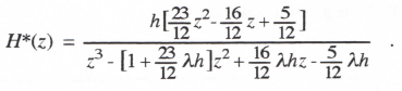

Here H*(z) has three poles because the denominator is a cubic in z. One of the poles corresponds to an equivalent characteristic root λ* which is almost equal to the ideal root λ, when |λh| << 1. The other poles represent characteristic roots which are extraneous. They result from the past two state-variable derivatives, f_n-1 and f_n-2, which are used in the AB-3 algorithm in addition to f_n. For small integration step sizes, i.e., |λh| << 1, the two extraneous roots cause transients that decay rapidly in comparison with e^λt for λ negative real. But they can cause instability as the integration step h gets larger. If we consider the case where z = -1 is a pole of H*(z) in Eq. (3.78) and solve for λh we find that λh = -6/11. Again, z = -1 corresponds to one of the extraneous roots and leads to an undamped transient at one-half the frame rate (sample frequency), 1/h. For any larger integration step size, corresponding to λh < -6/11, the digital system becomes unstable. For AB-3 integration the overall stability boundary in the complex λh plane is shown in Figure 3.2. This boundary is obtained by the same method used earlier for AB-2. Thus we set the denominator of Eq. (3.78) equal to zero with z = e^jθ and solve for λh as θ ranges between –π and π. Note in Figure 3.2 that the AB-3 stability boundary projects into the right-half λh plane. This means that a neutrally-stable continuous system with λ on the imaginary axis will actually result in a stable (i.e., damped) AB-3 simulation, since λh in this case falls within the AB-3 stability boundary. This conclusion is verified by reference to Eq. (3.55), which shows that for ζ = 0 and e_I positive (e_I = 3/8 for AB-3 Integration), the damping ratio ζ* of the digital simulation will be positive. Note also from Eq. (3.55) that for third-order integration algorithms (i.e., k = 3), the damping ratio error is of order h³ will predominant compared with the frequency error, which is of order h⁴ when ζ = 0.

To obtain the stability boundary in the case of AB-4 integration, we write the digital system Z transform that results when AB-4 is used to simulate the first-order linear system with characteristic root λ. In this case we obtain H*(z) by replacing s in the transfer function 1/(s – λ) with 1/H_I*, where H_I* for AB-4 integration is given by Eq. (3.75). In this way we obtain

(3.79)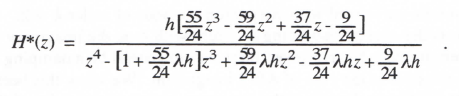

Here we see that H*(z) has four poles, three of which are extraneous. They result from the past three state-variable derivatives, f_n-1, f_n-2 and f_n-3, which are used in the AB-4 algorithm in addition to f_n. Again, for small integration step sizes, i.e., |λh| << 1, the three extraneous roots correspond to transients that decay rapidly in comparison with e^λt for λ negative real. But they can cause

3-18

instability as the integration step h gets larger. The overall stability boundary in Figure 3.2 for AB-4 integration is obtained by the same method used earlier for AB-2 and AB-3. Thus we set the denominator of Eq. (3.79) equal to zero with z = e^jθ and solve for λh as θ ranges between –π and π If we set the denominator equal to zero with z = -1 (this corresponds to θ = π in z = e^jθ) and solve for λh, we find that λh = -3/10. Thus AB-4 integration becomes unstable when the step size h is larger than -0.3/λ (we recall that λ must be negative for the continuous system to be stable). For h = -3/λ the digital system will be neutrally stable with an undamped transient at one-half the sample frequency due to the extraneous pole at z = -1. For this same step size, which is only 30 percent of the continuous-system time constant, -1/λ, the principal root λ* of the AB-4 simulation is within one percent of the ideal root λ!

Figure 3.3 illustrates the effect of the unstable extraneous root when the integrator step size is too large. Shown in the figure is the response of a first-order linear system to a unit step input as computed using AB-4 integration with an integrator step size h = 0.36. Since the system being simulated has a unit time constant, λ = -1 and λh = -0.36. Thus λh is outside the AB-4 stability boundary in Figure 3.2. The resulting instability is very apparent in Figure 3.3. At the same time we note that the AB-4 solution is very close to the exact solution until such time as the small initial transient associated with the unstable extraneous root grows to significant amplitude.

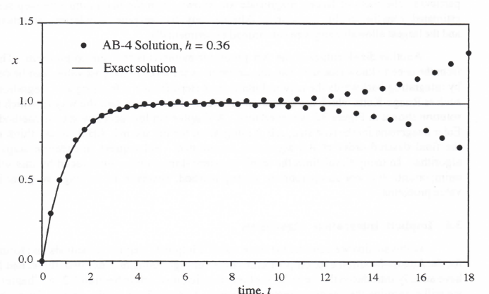
Figure 3.3. Unit step response of first-order system when simulated using AB-4 integration; the instability caused by one of the extraneous roots is evident.

Note in Figure 3.2 that the right side of the stability boundary for AB-4 integration appears to lie directly on the imaginary axis. In fact, this is very nearly true, which means that the damping ratio in simulating an undamped second-order system using AB-4 integration will be very nearly

3-19

equal to the ideal value of zero. In fact, reference to Eq. (3.56) for the damping ratio error e_ζ associated with integration methods of order k = 4 shows that the error is zero to order h⁴. The actual ζ* for ζ = 0 is of order h⁵, whereas the frequency error e_ω, is of order h⁴. In summary, for the simulation of undamped second-order systems Eqs. (3.53) through (3.56) show that the frequency error e_ω predominates when using integration algorithms of even order, and the damping ratio error e_ζ predominates when using integration algorithms of odd order.

From Figure 3.2 it is clear that the higher the order of the predictor integration method, the more restrictive is the upper limit on integration step size based on stability considerations. For real-time simulation, where dynamic accuracy requirements are often modest (0.1 to 1 percent), it is evident that AB-4 is unlikely to be a strong candidate algorithm due to instability considerations. This is especially true in simulating stiff systems, such as those containing controller subsystems with very short time constants. For adequate stability margin the AB-4 method requires the order of four integration steps per smallest time constant in the system being simulated. It is likely that such a small step size will produce a much more accurate solution than is needed. Yet any attempt to speed up the solution with even a modest increase in step size will lead to instability due to an extraneous root. In this case a lower order predictor method will give better results.

From the above discussion it is clear that the higher order AB methods should be used with some caution. However, if the characteristic roots of the linearized system are known and, in particular, the roots of largest magnitude are known, then the maximum safe step size can be estimated from the stability boundaries. Alternatively, the computer simulation can actually be run and the largest allowable step size determined experimentally.

Another disadvantage of the AB predictor methods is the startup problem. This results from the need to know past state-variable derivatives at t = 0. These past values can be determined by integrating backwards the required number of steps from t = 0, using an integration method such as Runge-Kutta which has no startup problem. This was in fact the way in which the AB-4 solution shown in Figure 3.3 was produced. A simpler but less accurate startup method is to use Euler integration for the first step, AB-2 integration for the second, AB-3 for the third, etc., until the final desired order of AB algorithm is attained. Subsequent integration steps use that algorithm. In many simulations the small transient startup errors introduced by this scheme are unimportant. It is not an appropriate startup method, however, in solving two-point boundary value problems.

3.5 Implicit Integration Algorithms

In this section we consider the three specific implicit integration methods that form the basis for the Adams-Moulton explicit predictor-corrector algorithms of order two, three, and four. We have already introduced the formulas for these implicit methods in Section 1.2 of Chapter 1. Here we will determine the integrator error coefficient, e_I, as defined by Eq. (3.37), for each method. This will, in turn, let us apply the formulas developed in Section 3.3 for the characteristic root and transfer function errors. Note that these implicit methods can be converted into explicit, single-pass methods in the simulation of linear systems, as will be described in Chapter 6.

The first of the three implicit methods is trapezoidal integration, given earlier in Eq. (1.8). When used to solve the first-order equation dx/dt = u(t), the difference equation becomes

3-20

(3.80)

Taking the Z transform and solving for H_I*, we obtain

(3.81)

Replacing z with e^jωh in Eq. (3.81), we obtain H_I* (e^jωh), the trapezoidal integrator transfer function for sinusoidal inputs. Thus

or

(3.82)

 

Noting that tan y = y + ³/3 + ^… , we can rewrite Eq. (3.82) as

(3.83)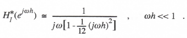

Comparison with Eq. (3.37) shows that the integrator error coefficient e_I = -1/12 and k = 2. Earlier, based on Eq. (3.36), we determined that e_I = 5/12 for AB-2 integration. Thus it is clear that trapezoidal integration is five times more accurate than AB-2 integration for small integration step sizes. From Section 3.3 we know that this accuracy comparison applies as well to characteristic root errors and transfer function gain and phase errors. The trapezoidal method has the further advantage that it does not introduce any extraneous roots. However, it cannot be used directly as a single-pass method in the solution of nonlinear differential equations because of the implicit nature of the algorithm.

In Eq. (1.15) we introduced a third-order implicit algorithm, which takes the following form in integrating the equation dx/dt = u(t):

(3.84)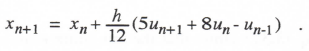

Taking the Z transform and solving for H_I*, we obtain

(3.85)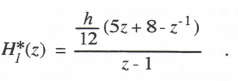

3-21

Again, the integrator transfer function for sinusoidal inputs is H_I*(e^jωh), which has the following asymptotic form when the exponential functions are expanded in power series and terms to order h⁴ are retained:

(3.86)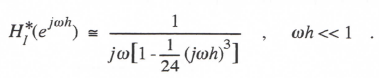

Comparison with Eq. (3.37) shows that the integrator error coefficient e_I = -1/24 and k = 3 for this third-order implicit integration algorithm. On the other hand Eq. (3.73) shows that e_I = 3/8 for AB-3 integration. Thus the third-order implicit method is nine times more accurate than the third-order predictor method for small integration step sizes. But the implicit method can only be used explicitly, i.e., without time-consuming iterations, when the system being simulated is linear. Also, it introduces one extraneous root for each state variable in the system being simulated. This is because the algorithm depends on a past derivative. Despite the presence of the extraneous root, however, instability occurs only for relatively large integration steps. For example, when the third-order implicit algorithm is used to simulate a system which has a negative real root λ, the simulation becomes unstable only when |λh|>6. This is a very large step indeed, and should not be a significant deterrent in the selection of this third-order method.

Finally, we consider the fourth-order implicit algorithm given in Eq. (1.17). When used to solve the equation dx/dt = u(t), it takes the form

(3.87)

Taking the Z transform and solving for H_I* we obtain

(3.88)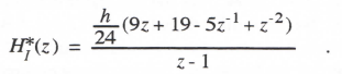

As noted previously, the integrator transfer function for sinusoidal inputs is H_I*(e^jωh). When the exponential functions are expanded in power series and terms to order h⁵ are retained, the following asymptotic formula for the integrator transfer function is obtained:

 

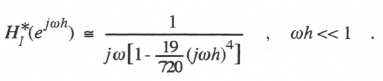
(3.89)

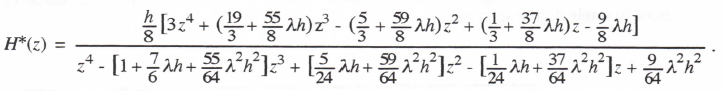
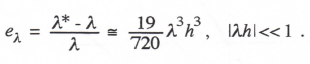
Comparison with Eq. (3.37) shows that the integrator error coefficient e_I = -19/720 and k = 4 for this fourth-order implicit integration algorithm. For AB-4 integration we found in Eq. (3.76) that e_I = 251/720. Thus the fourth-order implicit method is 251/19 or 13.2 times more accurate than the AB-4 predictor method for small integration step sizes. Again, the implicit method can only be used as an explicit algorithm in the simulation of linear systems. Also, it introduces two extraneous roots for each state variable in the system being simulated. This is because the algorithm depends on two past derivatives. These extraneous roots do not, however, cause significant stability problems for large integration steps. For example, when the system being

3-22

simulated has a negative real root λ, the simulation becomes unstable only when |λh| > 3. This represents a step size equal to three times the time constant associated with the negative real root.

Next we consider the overall stability boundaries in the λh plane for the implicit methods. When trapezoidal integration is used to simulate the first-order system with transfer function H(s) = 1/(s – λ), the digital system Z transform can be obtained by replacing s in H(s) with 1/H_I*(z), as given in Eq. (3.81). Thus

(3.90)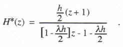

Setting the denominator of H*(z) equal to zero and solving for the pole z, we obtain

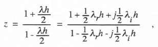
(3.91)

Where λ = λ_r + jλ_i. For the case where the characteristic root λ lies on the imaginary axis in the λh plane, λ_r = 0 and Eq. (3.91) becomes

 

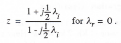
It follows for λ_r = 0 that |z| = 1, which means that the unit circle in the z plane corresponds to the imaginary axis in the λh plane. Thus the stability boundary for trapezoidal integration is the imaginary axis in the λh plane, and the stable region consists of the entire left-half plane. We conclude that when trapezoidal integration is used to simulate a stable linear system (λ in the left-half plane), the resulting simulation will be stable regardless of the step size h.

To obtain the stability boundaries in the λh plane for third and fourth-order implicit integration, we follow the procedure used earlier for the AB methods. In this way we obtain the stability boundaries shown in Figure 3.4. As noted above, the stability boundary for the second-order implicit method, i.e., trapezoidal integration, is the imaginary axis, with the stability region consisting of the entire left-half plane. As in the case of the stability regions for AB integration shown in Figure 3.2, we note in Figure 3.4 that the stability region in the λh plane shrinks as the algorithm order increases. Note also that the stability boundary for the fourth-order implicit method approaches the imaginary axis more closely than the boundary for the third-order method. This means that the damping ratio error in simulating either an undamped or lightly-damped second-order system will be less for the method of order four. Again this is consistant with Eqs. (3.55) and (3.56), which show that when the integration algorithm order k = 4 and ζ = 0 for the continuous system, the damping ratio error e_ζ is zero to order h⁴ and the frequency error predominates. Conversely, when the algorithm order k = 3 and ζ = 0 for the continuous system, the damping ratio error is finite to order h³ and predominates over the frequency error, which is zero to order h³. As noted earlier, the above conclusions hold for all single pass (or equivalent single-pass) integration methods.

3-23

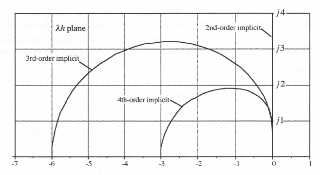
Figure 3.4 Stability boundaries for implicit integration methods.

3.6 Runge-Kutta Integration Algorithms

Next we consider the Runge-Kutta multiple-pass integration methods introduced in Section 1.2. We consider first a version of RK-2 known as Heun’s method, which from Eqs. (1.25) and (1.26) takes the following form when solving the differential equation given by Eq. (3.1):

(3.92)

(3.93)

Here _n+1 is an estimate of x_n+1 based on Euler integration. Taking the Z transform of Eqs. (3.92) and (3.93) with x₀ = 0 and solving for H*(z) = X*(z)/U*(z), we obtain

(3.94)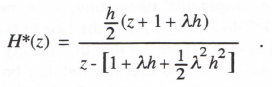

As noted in Eq. (2.22), the pole of H*(z), z₁ = 1 + λh + λ²h²/2, is related to the equivalent characteristic root, λ*, by the formula z₁ = e^λ*h. The asymptotic formula for λ* for |λh| << 1 can be found with the same procedure used earlier in Sections 3.2 and 3.3. Thus we set the denominator of H*(z) equal to zero with z replaced by e^λ*h, expand the exponential function in a power series with terms retained up to order h³, and solve for λ*. In this way we obtain

(3.95)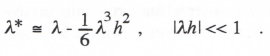

3-24

This equation is valid for both real and complex λ. The fractional error in the characteristic root, e_λ, is given by

(3.96)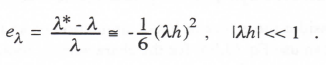

As expected for RK-2 integration, the error varies as the square of the integration step size h. Comparison of Eq. (3.96) with the result in Eq. (3.45) for single-pass integration methods suggests that e_I = 1/6 for RK-2 integration. Although the general single-pass transfer-function error formulas derived in Section 3.3 are not valid for the multiple-pass RK methods considered in this section, as we shall confirm shortly, the characteristic-root error formulas are valid. The reason for this will become apparent in the next section when we derive H*(z) for digital simulation of the first-order equation dx/dt = λx – u(t) using power-series integration.

Since e_I = 5/12 for AB-2 integration, it follows that the AB-2 root error is 2.5 times the root error of RK-2. On the other hand, the RK-2 algorithm requires two passes through the state equations per integration step. This means that RK-2 will in general take about twice as long to execute each integration step compared with AB-2. This results in double the step size for a given overall computation time and hence four times the root error, since both methods are second order. The net effect is to make the AB-2 root error 2.5/4 or 0.625 times the error when using RK-2 integration.

We next consider the transfer function for sinusoidal inputs, H*(e^jωh). This is obtained by substituting e^jωh for z in Eq. (3.94). Expanding e^jωh in power series and retaining terms up to order h² in the numerator and h³ in the denominator of H*, we can derive the following approximate formula for the fractional error in the transfer function:

or

(3.97)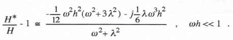

Again we note from Eqs. (1.53) and (1.54) that the real and imaginary parts of the right side of Eq. (3.97) are equal, respectively, to the approximate fractional gain error and phase error of the digital transfer function for sinusoidal inputs. Thus

(3.98)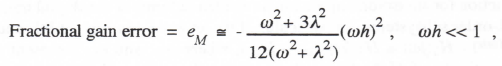

(3.99)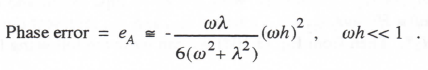

As expected, the transfer function gain and phase errors in RK-4 simulation of a first-order system vary as the square of the integration step size h. Note also that the result in Eq. (3.98) is different

3-25

from the result for e_M in Eq. (3.48) for e_I = 1/6 and k = 2. This confirms that the general transfer function error formulas for single-pass integration methods cannot be used for RK-2 integration.

Next we consider the errors in RK-2 simulation of an underdamped second-order linear system. Again we can use Eq. (3.95) for the characteristic root, λ*, with the complex λ given in terms of the undamped natural frequency ω_n and damping ratio ζ by Eq. (3.16). As noted above, for the characteristic root errors we can use for RK-2 integration the general result already derived in Eq. (3.54) for a single-pass algorithm with e_I = 1/6 and k = 2. Thus we find that

(3.100)

In considering the transfer function errors when RK-2 integration is used to simulate the second-order system given by Eq. (3.27), we take advantage of the result already obtained in Eq. (3.58) when the system being simulated is first order with transfer function given by 1/(s – λ). In this case the transfer function H(s) for the second-order system can be written as

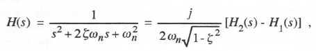
(3.101)

where

(3.102)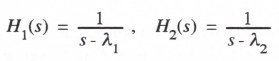

and the characteristic roots λ₁ and λ₂ are given by

(3.103)

From Eq. (3.101) it is clear that we can represent the Z transform of a digital system that is simulating an underdamped second-order system in terms of the sum of the Z transforms for two first-order simulations. Thus

(3.104)

where H_I*(z) and H₂*(z) are the Z transforms for the digital simulations of H₁(s) and H₂(s), respectively, as defined in Eq. (3.102). It follows that the error, H*(e^jωh) – H(jω), in the digital transfer function for sinusoidal inputs can be written in terms of the digital transfer function errors for the first-order subsystems. In particular, if we let λ = λ₁ in Eqs. (3.98) and (3.99), it follows that H₁*(e^jωh) – H₁(jω) H₁(jω)(eM₁+jeA₁), where eM₁ and eA₁ represent the gain and phase errors, respectively, of H₁*. Similarly, with λ = λ₂ in Eqs. (3.98) and (3.99), it follows that H₂*(e^jωh) – H₂(jω) H₂(jω)(eM₂ + jeA₂), where eM₂ and eA₂ represent the gain and phase errors, respectively, of H₂*. Then from Eq. (3.104) we can write the following formula for H*(e^jωh) – H(jω):

3-26

(3.105)

Eq. (3.105) is then divided by H(jω) to obtain H*/H – 1, the fractional error in digital transfer function. This then leads directly to the following formulas for the real and imaginary parts of H*/H – 1 i.e., the fractional error in transfer function gain, e_M, and the phase error, e_A, when RK-2 integration is used to simulate a second-order system:

(3.106)

(3.107)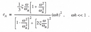

Note that the result in Eqs. (3.106) is different from the result for e_M in Eq. (3.60) for e_I = 1/6 and k = 2. Again, this shows that the general transfer function error formulas for single-pass integration methods cannot be used for RK-2 integration.

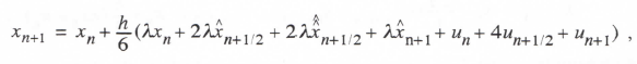
Before considering RK integration methods of higher order, we examine the real-time RK-2 algorithm introduced in Chapter 1. Like conventional RK-2 integration, real-time RK-2 is a two-pass method that employs Euler integration for the first pass. But the first pass is actually only a half step, i.e., it uses Euler integration to compute an estimate of the state halfway through the step. This estimate is then used to compute the derivative halfway through the step, which in turn is used in an Euler formula to compute the state at the end of the step. Applying the real-time RK-2 method, as defined in Eqs. (1.27) and (1.28), to the first-order system given by Eq. (3.1) leads to the following difference equations:

(3.108)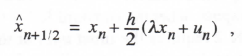

(3.109)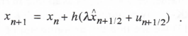

Using a sample period T = h/2, we can rewrite Eqs. (3.108) and (3.109) as the following single difference equation:

(3.110)

Taking the Z transform, replacing T with h/2, and solving for H*(z) = X*(z)/U*(z), we obtain

3-27

(3.111)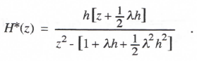

We determine the equivalent characteristic root λ* of the digital system by setting the denominator of Eq. (3.111) equal to zero with z = e^λ*T = e^λ*h/2. Then z² = e^λ*h and the denominator of H* in Eq. (3.111) becomes the same as the denominator of H* in Eq. (3.94) for the standard RK-2 with z = e^λ*h. Thus λ* for real-time RK-2 is the same as λ* for standard RK-2 and the characteristic root errors given by Eqs. (3.96) and (3.100) apply for either RK-2 method.

To obtain the digital transfer function for sinusoidal inputs we replace z with e^jωT = e^jωh/2 in Eq. (3.111). Expanding the exponential functions in power series and retaining terms up to order h³, we derive the following asymptotic formulas for the transfer function fractional gain and phase errors:

(3.112)

(3.113)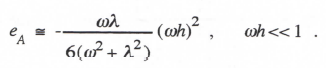

Comparison with Eq. (3.98) for standard RK-2 shows that the gain error, e_M, for real-time RK-2 is less than half as large. This improved accuracy results from the fact that u_n and u_n+1/2 serve as inputs for the nth integration frame in real-time RK-2 integration. This means that the input is sampled at twice the integration frame rate. In standard RK-2 the inputs for the nth integration frame are u_n and u_n+1, which represents an input sample rate equal to the integration frame rate.

The transfer function gain and phase errors for real-time RK-2 simulation of second-order linear subsystems are obtained using the same procedure employed to get Eqs. (3.106) and (3.107) for standard RK-2 integration. The formulas are given in Table 3.2 at the end of this chapter. Comparison with the formulas for standard RK-2 shows that the phase errors are identical. However, the gain error for real-time RK-2 is at least a factor of two smaller. Again, this can be ascribed to the doubled input sampling rate in the case of real-time RK-2.

In addition to providing better transfer-function gain accuracy, the real-time RK-2 method is compatible with real-time inputs, whereas standard RK-2 (Heun’s method) is not. As pointed out in Section 1.2, standard RK-2 requires the input u_n+1 at the start of the second pass, halfway through the nth integration frame, before u_n+1 is available in real time. Halfway through the nth integration step, real-time RK-2 only requires u_{n + 1/2}, which has just become available in real-time. From Eqs. (3.94) and (3.111) we see that the denominator of H*(z) is the same for both RK-2 methods when simulating the continuous system given by H(s) = 1/(s – λ). It then follows that the stability region in the λh plane will be identical for both methods. Later in this section we will examine the stability regions for all the RK algorithms considered here.

We now consider the RK-3 algorithm defined by Eqs. (1.35), (1.36) and (1.37) in Section 1.2. When applied to the first-order linear system described by Eq. (3.1), the method results in the following difference equations:

3-28

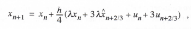
where

(3.114)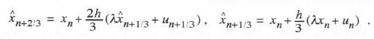

Using a sample period T = h/3, we can rewrite Eq. (3.114) as the following single difference equation:

(3.115)

Taking the Z transform, replacing T with h/3, and solving for H*(z) = X*(z) / U*(z), we obtain

(3.116)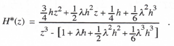

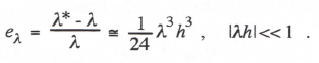
We determine the equivalent characteristic root λ* by setting the denominator of H* equal to zero with z = e^λ*T = e^λ*h/3. Expanding the exponential functions in power series and retaining terms to order h⁴, we obtain the following asymptotic formula for the characteristic root error, e_λ:

(3.117)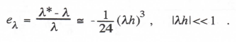

As expected for RK-3 integration, the error varies as the cube of the integration step size h. Comparison of Eq. (3.117) with the result in Eq. (3.45) for single-pass integration methods suggests that e_I = 1/24 for RK-3 integration. Again we note that the general single-pass transfer-function error formulas derived in Section 33 are not valid for the multiple-pass RK methods, but the characteristic-root error formulas are valid. Thus we can immediately write from Eq. (3.55) with k = 3 and e_I = 1/24 the formulas for the RK-3 root errors when the continuous system root λ is complex.

To obtain the digital transfer function for sinusoidal inputs we replace z with e^jωT = e^jωh/3 in Eq. (3.116). Expanding the exponential functions in power series and retaining terms up to order h⁴, we derive the following asymptotic formulas for the transfer function fractional gain and phase errors:

(3.118)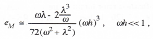

(3.119)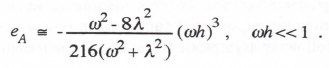

The transfer function gain and phase errors for RK-3 simulation of second-order linear subsystems are obtained using the same procedure employed to get Eqs. (3.106) and (3.107) for RK-2 integration. The formulas are given in Table 3.2 at the end of this chapter.

3-29

Finally, we consider the RK-4 integration algorithm defined by Eqs. (1.38) through (1.41) in Chapter 1. When applied to the first-order linear system described by Eq. (3.1), the method results in the following difference equations:

Where

(3.120)

Using a sample period T = h/2, we can rewrite Eq. (3.120) as the following single difference equation:

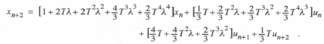
(3.121)

Taking the Z transform, replacing T with h/2, and solving for H*(z) = X*(z) /U*(z), we obtain

(3.122)

As before, we determine the equivalent characteristic root λ* by setting the denominator of H* equal to zero with z = e^λ*T = e^λ*h/2. Expanding the exponential functions in power series and retaining terms to order h⁵, we obtain the following asymptotic formula for the characteristic root error, e_λ:

(3.123)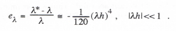

As expected for RK-4 integration, the error varies as the fourth-power of the integration step size h. Comparison of Eq. (3.123) with the result in Eq. (3.45) for single-pass integration methods suggests that e_I = 1/120 for RK-4 integration. Once more we note that the general single-pass characteristic-root error formulas derived in Section 3.3 are valid for the multiple-pass RK methods, but the transfer-function error formulas are not. Thus we can immediately write from Eq. (3.56) with k = 4 and e_I = 1/120 the formulas for the RK-4 root errors when the continuous system root λ is complex.

To obtain the digital transfer function for sinusoidal inputs we replace z with e^jωT = e^jωh/2 in Eq. (3.122). Expanding the exponential functions in power series and retaining terms up to order h⁵, we derive the following asymptotic formulas for the transfer function fractional gain and phase errors:

3-30

(3.124)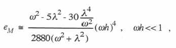

(3.125)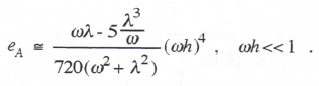

The transfer function gain and phase errors for RK-4 simulation of second-order linear subsystems are obtained using the same procedure employed to obtain Eqs. (3.106) and (3.107) for RK-2 integration. The formulas are given in Table 3.2 at the end of this chapter.

It is apparent in this section that the Runge-Kutta algorithms enjoy a significant advantage over the Adams-Bashforth predictor algorithms of the same order for a given integration step size. However, this advantage is more than offset by the additional RK execution time that results from multiple passes per integration step. For example, for AB-4 integration the fractional error in characteristic root is given by e_λ – (251/(720)(λh)⁴, whereas from Eq. (3.123) for RK-4 we see that e_λ-(1/(120)(λh)⁴ = -(6/(720)(λh)⁴ . Thus e_λ for AB-2 integration is 251/6 times e_λ for RK-4 integration. On the other hand, since RK-4 is a four-pass method, it will take approximately four times as long to execute one overall integration step in comparison with the single-pass AB-4 method. For the same overall solution time using a given processor this means that the mathematical step-size h for RK-4 must be four times the step size h for AB-4. Since e_λ varies as h⁴ for both algorithms, the error in e_λ for AB-4 will be 251/(6×4⁴), or 251/1536) times e_λ for RK-4. Thus AB-4 is in fact more accurate than RK-4 for a given computer speed.

Another disadvantage of RK-4, as noted in Chapter 1, is its incompatibility with real-time inputs. On the other hand, we have noted that the AB algorithms present startup problems. They also perform poorly in response to discontinuous inputs and generate extraneous roots which can cause instabilities if the step size h is made too large. Even though RK methods introduce no extraneous roots, it is nevertheless important to examine the region of stability in the λh plane. This is accomplished by using the same method employed in Section 3.4 for AB integration. Thus we calculate the values of λh for which the pole of H*(z) lies on the unit circle in the z plane. In particular, we let z = e^jθ in the denominator of H*(z) and solve for λh as the polar angle θ varies between –π and +π. Application of this procedure to H*(z) as given in Eqs. (3.94), (3.116) and (3.122) for RK-2, 3 and 4, respectively, leads to the stability boundaries shown in Figure 3.5. Values of λh lying within these boundaries correspond to stable digital solutions.

Comparison of Figure 3.5 with Figure 3.2 shows that the stability regions for RK integration are much larger than those for AB integration. Note also that the higher the order of the RK method, the larger the stability region. This is exactly the reverse of AB integration, where the stability region gets smaller as the algorithm order is increased. As in the case of accuracy comparisons, however, it is important to take into account the execution speeds of the different algorithms in comparing stability regions. From this viewpoint, we should reduce the stability regions for the multiple-pass RK-2, 3 and 4 algorithms by factors of 2, 3 and 4, respectively, when comparing them with the stability regions for the single-pass AB algorithms. This has been done in Figure 3.6, where the stability boundaries for AB integration are also shown. From the figure it is evident that the RK stability regions, even when normalized to account for multiple

3-31

passes, still are larger than the AB-2 regions. This is especially true in the case of 3rd and 4th-order algorithms.

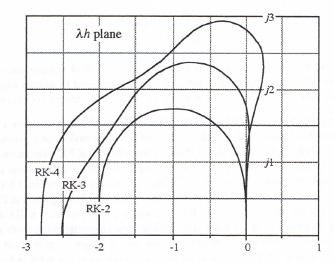
Figure 3.5. Stability regions for Runge-Kutta integration algorithms.

Figure 3.6. Comparison of normalized Runge-Kutta stability regions with Adams-
Bashforth stability regions.

3-32

3.7 Power Series Integration Algorithms

When the derivatives of the state variables are functions that can be differentiated analytically, then the following power-series algorithm can be used for numerical integration of the state equation, dx/dt = f:

(3.126)

The order of the integration method depends on the number of terms utilized before the power series is truncated. Halin has been particularly successful in exploiting the power series method as an effective means of integrating nonlinear differential equations.* This type of integration is often used with variable-order integration formulas as well as variable step size. However, we will assume here that both the algorithm order and step size are fixed, and that the nonlinear differential equations have been linearized so that we can use the method of Z transforms to analyze the dynamic errors. The results of this analysis will give us insight into the dynamic performance of the power series method compared with other integration algorithms.

Taking the Z transform of Eq. (3.126) and assuming that x₀ = 0, we obtain

(3.127)

To derive the power series integrator transfer function for a sinusoidal input data sequence, we replace z by e^jωh and note that f_n = e^jωnh, _n = jωe^jωnh = jωf_n, _n = (jω)²f_n,, etc. It then follows that Eq. (3.127) becomes

Solving for X*/F* = H_I*, the power series integrator transfer function, we obtain

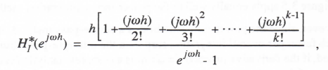
(3.128)

where we have truncated the power series at the h^k-1 term. Expanding e^jωh in a power series and retaining terms to order h^k , we obtain the following asymptotic formula for the power series integrator transfer function:

(3.129)

* See, for example, Halin, H.J., “Integration Across Discontinuities in Ordinary Differential Equations Using Power Series,” Simulation, Vol. 32, No. 2, February, 1979, pp 33-45.

3-33

Comparison with Eq. (3.37) shows that the kth-order power series integration algorithm has an integrator error coefficient, e_I, given by

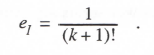
(3.130)

Since the power series integration algorithm is a single-pass method, the value of e_I in Eq. (3.130) can be used directly in all the asymptotic formulas of Section 3.3 for characteristic root errors, and for transfer function gain and phase errors.

To determine the stability region in the λh plane for power series integration, we apply the method to the first-order system given by Eq. (3.1) with the input u(t) = 0, i.e., dx/dt = f = λx. Noting that ḟ = λẋ = λ²x, = λ³x, etc., we can write the difference equation as

(3.131)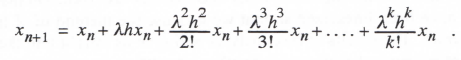

Here we have assumed a power series integration algorithm of order k. Taking the Z transform and solving for X*(z), we obtain

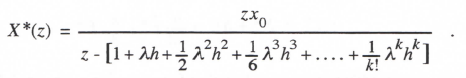
(3.132)

Comparison of the denominator of X*(z) in Eq. (3.132) for k = 2, 3 and 4 with the denominator of H*(z) in Eqs. (3.94), (3.116) and (3.122) for RK-2, 3 and 4 integration, respectively, we see that they are identical for the same k. Since the roots of the denominator of the Z transform determine the equivalent roots λ* of the digital simulation, it follows that the equivalent characteristic roots λ* for power series integration of order k are identical with the roots λ* for RK integration of order k when simulating the same linear system. It also follows for a given integration order k that the stability regions in the λh plane will be identical for the two methods. Thus the stability regions in Figure 3.5 apply equally well to the power series integration method.

However, since the power series method is a single-pass method, it is possible that it will execute much faster per overall integration step than the multiple-pass Runge-Kutta methods. On the other hand, if the derivative function f = dx/dt is a complex analytic function, the calculation of the derivatives of f may be very intensive, especially for a large order k of integration algorithm. This will slow down the power series method, so that it is not easy to draw general conclusions on which method will be faster. The speed tradeoff will be very problem dependent. Note also that it may be difficult, if not impossible, to apply the power series method to real time simulation, since the required higher derivatives of the real-time inputs will not in general be available. Furthermore, many real-time simulations involve derivative functions that are represented by multi-dimensional data tables rather than analytic functions. In this case it does not appear that the power series method is a candidate integration algorithm, since the required state-variable derivatives do not exist. Nevertheless, power series integration methods can be very efficient for simulating particular types of differential equations.

3-34

3.8 Adams-Moulton Predictor-corrector Algorithms

In Chapter 1 we noted that the AB predictor algorithms can be combined with implicit algorithms to mechanize the AM (Adams-Moulton) predictor-corrector integration algorithms. In this section we consider the AM-2, 3 and 4 methods in regard to characteristic root errors, and transfer-function gain and phase errors. We will also consider the extraneous roots introduced by these methods, as well as their overall stability region in the λh plane.

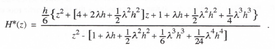
First we consider the second-order predictor-corrector method, AM-2. In Eqs. (1.19) and (1.20) the general form of the equations is presented. When we apply these equations to the first-order linear system given by Eq. (3.1), the following single difference equation is obtained:

(3.133)

Taking the Z transform and solving for H*(z) = X*(z)/U*(z), we have

(3.134)

The two poles of H*(z) (i.e., the two roots of the denominator), z₁ and z₂, determine the equivalent characteristic roots. One of the two roots corresponds to the ideal characteristic root, λ, in accordance with the formula z₁ = e^λ*h. Here λ*, as before, represents the equivalent characteristic root of the digital system. Since the denominator of H*(z) in Eq. (3.134) is a quadratic in z, we can solve analytically for the two poles, z₁ and z₂, and thus determine the exact value of λ* as well as the exact value of the equivalent extraneous root. As noted earlier in Section 3.4, this extraneous root results from the dependence of x_n+1 in the predictor formula on x_n-1 as well as x_n. A simple approximate analytic formula for the principal root λ* is obtained by replacing z with e^λ*h in the denominator of H*(z), expanding e^λ*h in a power series with terms to order h³ retained, and solving for λ*. When this is done, the formula for λ* and hence the fractional root error, e_λ, agrees exactly with the result for 2nd-order implicit (i.e., trapezoidal) integration as given by Eq. (3.45) with e_I = -1/12. Thus

(3.135)

Since e_λ = -(5/12)λ²h² for AB-2 integration, it follows that the characteristic root error for AB-2 is 5 times the error for AM-2 integration. On the other hand, the AM-2 algorithm requires two passes through the state equations per integration step. This means that AM-2 will in general take about twice as long to execute each integration step compared with AB-2. This results in double the step size for a given overall computation time and hence four times the root error, since both methods are second order. The net effect is to make the AB-2 root error 5/4 or 1.25 times the AM-2 error. On that basis we conclude that AM-2 enjoys a slight edge over AB-2 as a second-order algorithm. But AM-2 does have the disadvantage in real-time simulation of requiring the input u_n+1 for the second pass one-half frame before it is available in real time. As we shall see in the next section, this difficulty is removed in the real-time AM-2 predictor-corrector method.

3-35

As explained in the introductory paragraph of Section 3.3, the reason that the asymptotic error formulas developed for all single-pass integration algorithms, including implicit methods, apply equally well to the two-pass AM methods is that the local truncation error associated with the predictor pass is of order k +1 and therefore does not contribute to the global error of order k for the overall algorithm. In other words, to order h^k it makes no difference whether the exact x_n+1 or the estimate _n+1 is used for the corrector formula in the second AM-2 pass. Thus the asymptotic formulas for characteristic root and transfer function errors when using AM-2 integration are identical with those noted earlier in Section 3.5 for the implicit methods. The errors are given by the single-pass formulas of Section 3.3 with e_I = -1/12, -1/24 and -19/720, respectively, for AM-2,3 and 4 integration.

It follows, therefore, that the approximate asymptotic formulas (valid when ωh << 1) for transfer function gain and phase errors when using AM-2 integration to simulate Eq. (3.1) are given by Eq. (3.48) with e_I = -1/12 and k = 2. Of course, the exact transfer function formula is still given by Eq. (3.134) with z replaced by e^jωh. Note that H*(z) in Eq. (3.134) for AM-2 is not the same as H*(z) for trapezoidal in Eq. (3.90), even though the asymptotic formulas for transfer function gain and phase errors are the same.

We can determine H*(z) for AM-3 when used to simulate the first-order system represented by H(s) = 1/(s – λ) by applying Eqs. (1.21) and (1.22) to Eq. (3.1), rewriting the result as a single difference equation, and taking the Z transform. When this is done, the following formula is obtained:

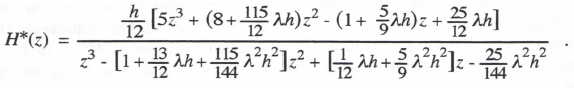
(3.136)

For a given λh the three poles of H*(z) can be used to calculate the equivalent characteristic roots for the digital system. One of these roots, λ*, corresponds to the ideal root, λ. The other two roots are extraneous. As noted above, the asymptotic formula for e_λ, the fractional root error, is identical to the value for 3rd-order implicit integration and is therefore given by Eq. (3.45) with e_I = -1/24 and k = 3. Thus for AM-3

(3.137)

Since e_λ = – (3/8)λ³h³ for AB-3 integration, it follows that the characteristic root error for AB-3 is 9 times the error for AM-3 integration. However, we again note that the AM-3 algorithm requires two passes through the state equations per integration step. This means that AM-3 will in general take approximately twice as long to execute each integration step compared with AB-2. This results in double the step size for a given overall computation time and hence eight times the root error, since both methods are third order. The net effect is to make the AB-3 root error 9/8 or 1.125 times that of AM-3. On that basis we conclude that AM-3 has a slight edge over AB-3 as a third-order algorithm, except for its incompatibility with real-time inputs. Again, in the next section we will consider a real-time version of the AM-3 predictor-corrector method.

The approximate asymptotic formulas for transfer function gain and phase errors when using AM-3 integration to simulate Eq. (3.1) are given by Eq. (3.47) with e_I = – 1/24 and k = 3.

3-36

The exact transfer function formula is given by Eq. (3.136) with z replaced by e^jωh. Again we note that H*(z) in Eq. (3.136) for AM-3 is not the same as H*(z) for third-order implicit integration, even though the asymptotic formulas for transfer function gain and phase errors are the same.

Finally, we consider AM-4 simulation of the first-order system with H(s) = 1/(s – λ). By applying Eqs. (1.23) and (1.24) to Eq. (3.1), rewriting the result as a single difference equation, and taking the Z transform, we obtain the following formula for H*(z):

(3.138)

For a given λh the four poles of H*(z) can be used to calculate the equivalent characteristic roots for the digital system. One of these roots, λ*, corresponds to the ideal root, λ. The other three roots are extraneous. Again, the asymptotic formula for e_λ, the fractional root error, is identical to the value for 4rd-order implicit integration and is therefore given by Eq. (3.45) with e_I = -19/720 and k = 4. Thus for AM-4

(3.139)

Since e_λ = -(251/720)λ³h³ for AB-4 integration, it follows that the characteristic root error for AB-4 is 251/19 or 13.2 times the error for AM-4 integration. However, we note once again that the AM-4 algorithm requires two passes through the state equations per integration step. This means that AM-4 will in general take approximately twice as long to execute each integration step compared with AB-2. This results in double the step size for a given overall computation time and hence sixteen times the root error, since both methods are fourth order. The net effect is to make the AB-4 root error 13.2/16 or 0.826 times that of AM-4. On this basis AB-4 has a slight edge over AM-4 as a fourth-order algorithm, in addition to its compatibility with real-time inputs. In the next section we will consider a real-time version of the AM-4 predictor-corrector method which is more competitive with AB-4.

The approximate asymptotic formulas for transfer function gain and phase errors when using AM-4 integration to simulate Eq. (3.1) are given by Eq. (3.48) with e_I = -19/720 and k = 4. The exact transfer function formula is given by Eq. (3.138) with z replaced by e^jωh. Again we note that H*(z) in Eq. (3.138) for AM-4 is not the same as H*(z) for fourth-order implicit integration, even though the asymptotic formulas for transfer function gain and phase errors are the same.

We have already pointed out that the asymptotic formulas for characteristic root errors, and transfer function gain and phase errors, are the same for AM methods as for implicit methods of the same order. Thus Eqs. (3.54), (3.55) and (3.56) with e_I = -1/12, -1/24 and -19/720 for AM-2,3 and 4, respectively, give the formulas for frequency and damping ratio errors when AM integration is used to simulate systems with complex characteristic root pairs. Similarly, the

3-37

transfer function gain and phase errors for second-order subsystems are given by Eq. (3.59) for AM-3 and Eq. (3.60) for AM-2 and AM-4.

We now examine the stability regions in the λh plane for AM integration. The method used to generate the stability boundaries is the same as that used previously for AB, implicit and RK integration. Thus we let z = e^jθ (i.e., |z|=1) in the denominator of H*(z) in Eqs. (3.134), (3.136) and (3.138) for AM-2, 3 and 4, respectively. The denominators are then set equal to zero and λh is determined for values of the polar angle θ ranging between –π and π. In this way the stability boundaries shown in Figure 3.7 are obtained. Values of λh lying within the boundaries correspond to stable digital solutions.

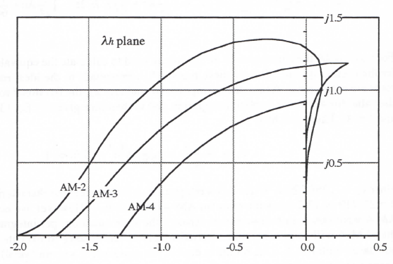
Figure 3.7. Stability boundaries for Adams-Moulton integration algorithms.

Comparison of Figure 3.7 with Figure 3.2 shows that the stability regions for AM methods are significantly larger than those for AB methods for algorithms of the same order k. However, as noted earlier in the comparison of stability regions of RK with AB, it is important to take into account the execution speeds of the different algorithms. From this viewpoint, we should reduce the stability regions for the two-pass AM-2, 3 and 4 algorithms by a factor of 2 when comparing them with the stability regions for the single-pass AB algorithms. This has been done in Figure 3.8, where the stability boundaries for AB integration are superimposed. From the figure it is evident that the stability region for AB-2 is in general larger than the normalized region for AM-2. The region for AB-3 is comparable with that for AM-3, with AM-3 permitting larger step sizes for real roots and AB-3 permitting somewhat larger step sizes for imaginary roots. Clearly the normalized stability boundary for AM-4 is significantly larger than the boundary for AB-4. After we analyze the real-time versions of the AM predictor corrector method in the next section, we will

3-38

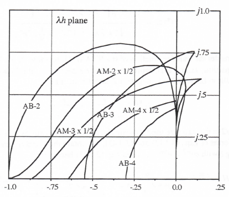
Figure 3.8. Comparison of normalized Adams-Moulton stability regions with Adams-Bashforth stability regions.

reexamine normalized stability boundaries for all methods of equal order k, as considered in this chapter.

3.9 Real-time Predictor-corrector Integration Algorithms

In Section 1.2 we introduced a variation of the AM predictor-corrector method which utilizes a half-step predictor algorithm for the first pass. Then the corrector pass is based on the resulting state-variable derivative at the half step, as well as the derivative at the beginning of the step and, depending on the algorithm order, derivatives at prior steps. In this case the predictor-corrector method is compatible with real-time inputs because, at the start of the second pass, the input u_n+1/2, which is available in real time, is required rather than u_n+1 , which is not yet available in real time. For this reason we identify the algorithm type as RTAM.

From Eqs. (1.29) and (1.30), for the case where RTAM-2 is used to simulate the first-order system described by Eq. (3.1), the difference equations become

(3.140)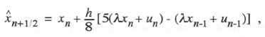

(3.141)

After writing Eqs. (3.140) and (3.141) as a single difference equation and taking the Z transform with the step size equal to h/2, we obtain the following formula for H*(z) = X*(z)/U*(z):

3-39

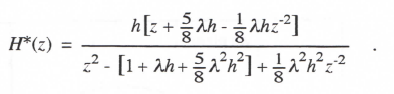
(3.142)

First we consider the transfer function of the RTAM-2 integrator. If we let λ = 0 in Eq. (3.1), the resulting equation, dx/dt = u(t), represents simple integration. It follows that letting λ = 0 in Eq. (3.142) results in the RTAM-2 integrator Z transform. Thus

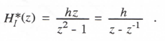
(3.143)

Since T = h/2 is the step size used to write the difference equations (3.140) and (3.141) and hence the Z transforms of Eqs. (3.142) and (3.143), we obtain the transfer function for sinusoidal inputs by replacing z with e^jωT = e^jωh/2. Then Eq. (3.143) becomes

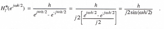
(3.143)

Eq. (3.143) represents the exact formula for the RTAM-2 integrator transfer function. If we expand sin(ωh/2)in a power series and retain only the first two terms, we obtain

(3.144)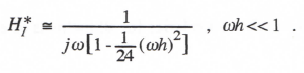

This is the asymptotic formula for the RTAM-2 integrator transfer function for small step size h. Comparison with Eq. (337) shows that the integrator error coefficient e_I = 1/24 and k = 2. We have already noted that the two-pass predictor-corrector algorithms exhibit asymptotic accuracy equivalent to single-pass methods. This is because the local truncation error of the predictor pass is of order h^k+1 and does not contribute to the global error of order h^k. Thus all the formulas of Section 3.3 for characteristic root errors as well as transfer function gain and phase errors apply equally well to RTAM-2 with e_I = 1/24 and k = 2. We recall that e_I = 5/12 for AB-2 integration and -1/12 for trapezoidal integration. Thus RTAM-2 is the most accurate of any of the second-order integration methods. From Eq. (3.45) the fractional error in characteristic root is given by

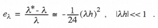
(3.145)

Since e_λ = – (5/12)λ²h² for AB-2 integration, it follows that the characteristic root error for AB-2 is 10 times the error for RTAM-2 integration. On the other hand, the RTAM-2 algorithm requires two passes through the state equations per integration step. This results in double the step size for a given overall computation time and hence four times the root error, since both methods are second order. The net effect is to make the AB-2 root error 10/4 or 2.5 times the error when RTAM-2 is used. On this basis we conclude that RTAM-2 enjoys a significant advantage over AB-2 as a second-order algorithm. This advantage will extend to characteristic root errors and

3-40

transfer function errors in general, in accordance with all of the single-pass error formulas derived in Section 3.3. Unlike AM-2, RTAM-2 also matches AB-2 in compatibility with real-time inputs, as noted above.

We consider next the third-order real-time predictor-corrector algorithm, RTAM-3, as defined in Eqs. (1.31) and (1.32). When applied to Eq. (3.1), the method results in the following difference equations:

(3.146)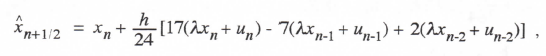

(3.147)

Writing Eqs. (3.146) and (3.147) as a single difference equation and taking the Z transform with the step size equal to h/2, we obtain the following formula for H*(z) = X *(z)/ U*(z):

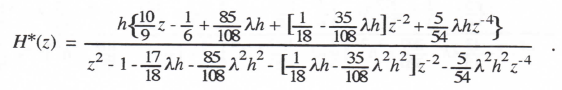
(3.149)

Consider the transfer function of the RTAM-3 integrator. If we let λ = 0 in Eq. (3.1), the resulting equation, dx/dt = u(t), represents simple integration. It follows that letting λ = 0 in. Eq. (3.148) results in the RTAM-3 integrator Z transform. Thus

(3.149)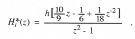

Since T = h/2 is the step size used to write the difference equations (3.146) and (3.147) and hence the Z transforms of Eqs. (3.148) and (3.149), we obtain the transfer function for sinusoidal inputs by replacing z with e^jωT = e^jωh/2. After expanding the exponential terms in power series and retaining terms up to order h⁴, we obtain the following asymptotic formula for the RTAM-3 integrator transfer function:

(3.150)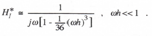

Comparison with Eq. (3.37) shows that the integrator error coefficient e_I = 1/36 and k = 3. All of the formulas for characteristic root errors and transfer function gain and phase errors, as derived in Section 3.3, are valid for RTAM-3 with these values for e_I and k. We recall that e_I = 3/8 for AB-3 integration and -1/24 for AM-3 integration. Thus RTAM-3 is the most accurate of the three third-order integration methods. The error coefficient e_I for AB-3 integration is (3/8)/(1/36) or 13.5 times larger. Because of the required two passes per integration step, the RTAM-3 method requires double the step size of AB-3 for a given overall computation time. This in turn reduces the accuracy by a factor of eight, since the method is third order. The net effect is to make the AB-3 errors 13.5/8 or 1.6875 times the error when RTAM-3 is used. On this basis we conclude that

3-41

RTAM-3 enjoys an accuracy advantage over AB-3 as a third-order algorithm. Unlike AM-3, RTAM-3 also matches AB-3 in compatibility with real-time inputs.

Finally, we consider the fourth-order real-time predictor-corrector algorithm, RTAM-4, as defined in Eqs. (1.33) and (1.34). When applied to Eq. (3.1), the method results in the following difference equations:

(3.151)

(3.152)

Writing Eqs. (3.151) and (3.152) as a single difference equation and taking the Z transform with the step size equal to h/2, we obtain the following formula for H*(z) = X * (z)/U*(z):

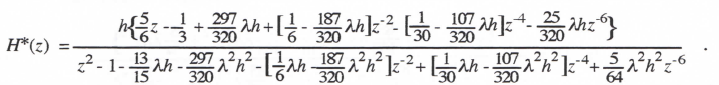
(3.153)

If we let λ = 0 in Eq. (3.1), the resulting equation, dx/dt = u(t), represents simple integration. It follows that letting λ = 0 in Eq. (3.148) results in the RTAM-4 integrator Z transform. Thus

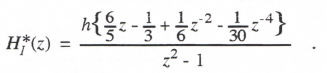
(3.154)

Since T = h/2 is the step size used to write the difference equations (3.151) and (3.152) and hence the Z transforms of Eqs. (3.153) and (3.154), we obtain the transfer function for sinusoidal inputs by replacing z with e^jωT = e^jωh/2. After expanding the exponential terms in power series and retaining terms up to order h⁵, we obtain the following asymptotic formula for the RTAM-3 integrator transfer function:

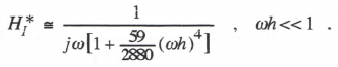
(3.155)

Comparison with Eq. (3.37) shows that the integrator error coefficient e_I = 59/2880 and k = 4. All of the formulas for characteristic root errors and transfer function gain and phase errors, as derived in Section 3.3, are valid for RTAM-4 with these vales for e_I and k. We recall that e_I = 251/720 or 1004/2880 for AB-4 integration and -19/720 or -76/2880 for AM-3 integration. Thus RTAM-4 is the most accurate of the three fourth-order integration methods. The error coefficient e_I for AB-4 integration is 1004/59 or 17.017 times larger. Because of the required two passes per integration step, however, the RTAM-4 method requires double the step size of AB-4 for a given overall computation time. This in turn reduces the accuracy by a factor of 2⁴ or 16, since the method is fourth order. The net effect is to make the AB-4 errors 17.017/16 or 1.064 times the error when RTAM-4 is used. On this basis we conclude that the accuracy of RTAM-4 is comparable with the accuracy of AB-4. Unlike AM-4, RTAM-4 also matches AB-4 in compatibility with real-time inputs.

We next examine the stability regions in the λh plane for RTAM integration. The method used to generate the stability boundaries is the same as that used previously for other integration methods. Thus we let z = e^jθ (i.e., |z| = 1) in the denominator of H*(z) in Eqs. (3.142), (3.148) and (3.153) for RTAM-2, 3 and 4, respectively. The denominators are then set equal to zero and λh is determined for values of the polar angle θ ranging between -π and π. In this way the stability boundaries shown in Figure 3.9 are obtained. Values of λh lying within the boundaries correspond to stable digital solutions. Comparison of Figure 3.9 with Figure 3.7 shows that the RTAM stability boundaries are somewhat larger than those for AM integration. Thus in addition to being more accurate and real-time-input compatible, the RTAM methods have better stability characteristics than standard AM integration methods. In a later section of this chapter we will examine the superimposed and normalized stability boundaries, grouped by order k, for all the algorithms considered in this chapter.

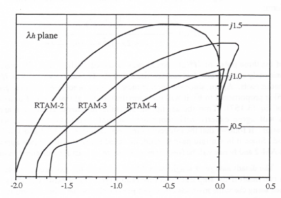
Figure 3.9. Stability boundaries for real-time Adams-Moulton integration algorithms.

3.10 Single-pass Predictor-corrector Algorithms

An interesting modification of the two-pass predictor-corrector integration methods considered in Sections 3.8 and 3.9 utilizes only derivatives based on the predicted values of the state-variables. Thus the second-order algorithm given earlier in Eqs. (1.19) and (1.20) becomes the following:

3-43

(3.156)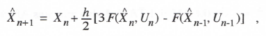

(3.157)

Since is the only new derivative that must be evaluated during the nth integration frame, having been evaluated in the previous frame, the algorithm requires only one evaluation of the state-variable derivative per integration frame. For this reason we call it a single-pass AM-2 method, abbreviated as SPAM-2. It will usually run approximately twice as fast as the conventional two-pass AM-2 algorithm. This is because the calculation of the state-variable derivative functions usually is the most intensive computational task in implementing the simulation of complex nonlinear systems, as we have already observed in comparing the execution speed of single and multiple-pass integration algorithms.

We next apply the single-pass AM-2 method given above by Eqs. (3.156) and (3.157) to the first-order linear system of Eq. (3.1). Taking the Z transform of the resulting difference equations and solving for X *(z)/U*(z), we obtain the following formula for the system Z transform:

(3.158)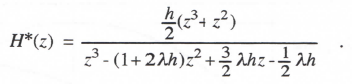

One of the three poles of H*(z) corresponds to the equivalent root, λ*, which for |λh| << 1 is approximately equal to the ideal characteristic root, λ. The other two poles of H*(z) correspond to extraneous roots. Again, since the local truncation error associated with the predictor pass in Eq. (3.156) is proportional to h³, it will not contribute to the global error of order h2 in the corrector pass of Eq. (3.157). Thus the asymptotic formulas for characteristic root and transfer function errors will agree exactly with those for standard, two-pass AM-2, as well as trapezoidal integration. It follows that the integrator error coefficient e_I = -1/12 and k = 2 for the SPAM-2 method. Since it is a single-pass method, as noted above it will execute approximately twice as fast as AM-2 and hence will be four times as accurate, at least for sufficiently small step size h.

The disadvantage of single-pass AM-2 lies with the extraneous roots and the instability which can result if the step size h becomes too large. The stability boundary in the λh plane is obtained using the same methods employed previously for the other integration algorithms. Thus we let z = e^jθ (i.e., |z| =1) in the denominator of H*(z) in Eq. (3.158). The denominator is then set equal to zero and λh is determined for values of the polar angle θ ranging between -π and π. In this way the stability boundary for SPAM-2 shown in Figure 3.10 is obtained. Also shown in the figure is the stability boundary for the single-pass RTAM-2 algorithm which we will discuss next. Comparison with Figure 3.7 for AM-2 and 3.9 for RTAM-2 shows that indeed the single-pass methods are much less stable. However, we must remember that the single-pass methods execute approximately twice as fast as the two-pass methods. Even when this is taken into account by shrinking the AM-2 and RTAM-2 stability boundaries by a factor of two, it is still evident that the single-pass methods are less stable.

Next we consider a single-pass version of the real-time AM-2 method introduced in the previous section. In the single-pass version of RTAM-2 the state-variable derivative, instead of being computed at both integer and half-integer frame times, as in Eqs. (1.29) and (1.30), is computed only at half-integer frame times based on a second-order predictor integration formula. The difference equations are the following:

(3.159)

(3.160)

Since is the only new derivative that must be evaluated during the nth integration frame, having been evaluated in the previous frame, the algorithm requires only one evaluation of the state-variable derivative per integration frame. For this reason we designate it as SPRTAM-2. It will usually run approximately twice as fast as the conventional two-pass AM-2 algorithm. Again, this is because the calculation of the state-variable derivative functions is the most intensive computational task in the simulation of complex nonlinear systems. Note that both RTAM-2 of Section 3.9 and SPRTAM-2, as given above in Eqs. (3.159) and (3.160), actually produce two outputs per integration step, and X_n+1. When we apply SPRTAM-2 to the first-order linear system of Eq. (3.1), rewrite the difference equations with a step size T = h/2, take the Z transform, and solve for X *(z)/U*(z), we obtain the following formula for H*(z), the digital system Z transform:

(3.161)

One of the three poles of H*(z) corresponds to the equivalent root, λ*, which for |λh| << 1 is approximately equal to the ideal characteristic root, λ. The other two poles of H*(z) correspond to extraneous roots. Once again, since the local truncation error associated with the predictor pass in Eq. (3.159) is proportional to h³, it will not contribute to the global error of order h² in the corrector pass of Eq. (3.160). Thus the asymptotic formulas for characteristic root and transfer function errors will agree exactly with those for the two-pass RTAM-2. It follows that the integrator error coefficient e_I = 1/24 and k = 2 for the SPRTAM-2 method. Since it is only a single-pass method, it will execute approximately twice as fast as RTAM-2 and hence will be 2² or 4 times more accurate, at least for sufficiently small step size h, when executed at maximum speed on a given computer.

As in the case of single-pass AM-2, the disadvantage of single-pass RTAM-2 lies with the extraneous roots and the instability which can result if the step size h becomes too large. The stability boundary in the λh plane is obtained from the denominator of H*(z) in Eq. (3.161) using the same methods employed previously for the other integration algorithms. The resulting stability boundary for single-pass RTAM-2 is shown in Figure 3.10. From the figure it is apparent that the stability region is somewhat larger than the region for single-pass AM-2. In addition, the single pass RTAM-2 is twice as accurate as single-pass AM-2, since e_I = 1/24 compared with -1/12.

Neither single-pass predictor-corrector algorithm is completely compatible with real-time inputs. In the case of single-pass AM-2 the derivative in Eq. (3.156) requires the input U_n+1 for the nth frame calculation, where it is clear that U_n+1 is not available in real time until the end of the frame. An alternative, of course, is to use the estimate as the real-time output, although this will be less accurate than the corrector output X_n+1. Similarly, in the case of single-pass RTAM-2 the derivative in Eq. (3.159) requires the input U_n+1/2 for the nth frame calculation, where U_n+1/2 is not available in real time until halfway through the frame. If the remaining half frame provides enough time to complete the calculation of and hence X_n+1, then the method is compatible with real time. Again, an alternative if this is not the case is to use the estimate as the real-time output, in which case the nth frame is considered to span the interval from t=(n-1/2)h to (n+1/2)h.

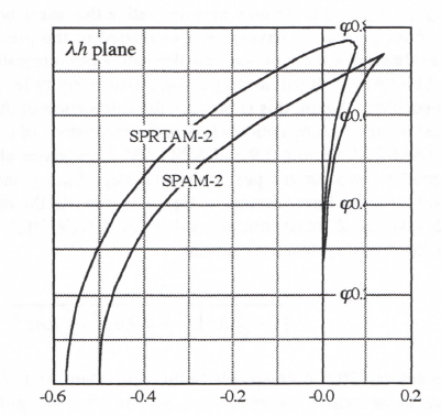
Figure 3.10. Stability boundaries for single-pass versions of AM-2 and real-time AM-2.

Higher-order single-pass predictor-corrector methods can also be considered. For single-pass AM-3 Eqs. (1.21) and (1.22) are replaced by

(3.162)

(3.163)

When we apply the above SPAM-3 algorithm to the first-order linear system of Eq. (3.1), take the Z transform and solve for X *(z)/U*(z), we obtain the following formula for H*(z), the digital system Z transform:

(3.164)

3-46

One of the four poles of H*(z) corresponds to the equivalent root, λ*, which for |λh|<< 1 is approximately equal to the ideal characteristic root, λ. The other three poles of H*(z) correspond to extraneous roots. The local truncation error associated with the predictor pass in Eq. (3.162) is proportional to h⁴ and will not contribute to the global error of order h³ in the corrector pass of Eq. (3.163). Thus the asymptotic formulas for characteristic root and transfer function errors will agree exactly with those for the two-pass AM-3. It follows that the integrator error coefficient e_I = -1/24 and k = 3 for the SPAM-3 method. Since it is only a single-pass method, it will execute approximately twice as fast as AM-3 and hence will be 2³ or 8 times more accurate, at least for sufficiently small step size h, when executed at maximum speed on a given computer.

The single-pass version of AM-4 is obtained by replacing X with everywhere in F(X , U) in Eqs. (1.23) and (1.24), which results in the following difference equations:

(3.165)

(3.166)

When we apply these difference equations to the first-order linear system of Eq. (3.1), take the Z transform, and solve for X *(z)/U*(z), we obtain the following formula for H*(z), the digital system Z transform:

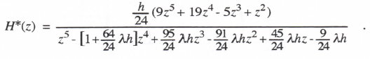
(3.167)

One of the five poles of H*(z) corresponds to the equivalent root, λ*, which for |λh|<< 1 is approximately equal to the ideal characteristic root, λ. The other four poles of H*(z) correspond to extraneous roots. The local truncation error associated with the predictor pass is proportional to h⁵ and will not contribute to the global error of order h⁴ in the corrector pass. Thus the asymptotic formulas for characteristic root and transfer function errors will agree exactly with those for the two-pass AM-4. It follows that the integrator error coefficient e_I = -19/720 and k = 4 for the SPAM-4 method. Since it is only a single-pass method, it will execute approximately twice as fast as AM-4 and hence will be 2⁴ or 16 times more accurate, at least for sufficiently small step size h, when executed at maximum speed on a given computer.

As in the case of single-pass AM-2, the disadvantage of single-pass AM-3 and AM-4 lies with the extraneous roots and the instability which can result if the step size h becomes too large. The stability boundaries in the λh plane are obtained from the denominator of H*(z) in Eqs. (3.164) and (3.167) using the same methods employed previously. Thus we let z = e^jθ (i.e., |z|= 1) in the denominator of H*(z), set the denominator equal to zero and solve for λh with the polar angle θ ranging between -π and π. The stability boundaries for single-pass AM-2, 3 and 4 are shown in Figure 3.11. Comparison with Figure 3.7 shows how much smaller the stability regions have become for single-pass predictor methods. However, we must again remind ourselves that the single-pass methods execute approximately twice as fast as the two-pass methods. Thus the stability regions of Figure 3.7 for conventional two-pass predictor-corrector methods should be reduced in size by a factor of two when comparing them with the regions in Figure 3.11 for the single-pass predictor-corrector methods. Even so, it is clear that single-pass predictor-corrector methods are less stable than two pass predictor-corrector methods of the same order.

As noted in the case of single-pass AM-2, the derivative in single-pass AM-3 and 4 requires the input U_n+1 for the nth frame calculation, when clearly U_n+1 is not available in real time until the end of the frame. When U is a real-time input, then, the estimate must be used as the real-time output, although this will be less accurate than the corrector output X_n+1.

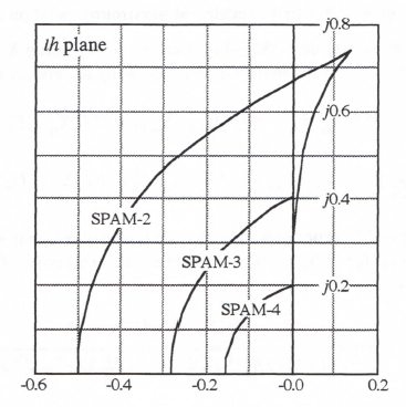
Figure 3.11. Stability boundaries for single-pass predictor-corrector (SPAM) integration algorithms.

For the third and fourth-order real-time predictor-corrector methods, RTAM-3 and RTAM-4, state-variable derivatives evaluated at both integer and half-integer frame times are required in the corrector pass, as can be seen in Eqs. (1.32) and (1.34). Thus it is not possible to construct a single-pass method with equivalent asymptotic accuracy for small step size h. One can derive a modified single-pass predictor-corrector method based only on derivatives at half-integer frame times, but the accuracy is less than that for the two-pass RTAM-3 and 4 algorithms.

3.11 Real-time Three-pass Predictor-corrector Algorithms

The performance of the two-pass RTAM-3 integration method suggests that a similar algorithm be used to provide an estimate of X_n+2/3 instead of X_n+1. Then a third pass based on F_n and F_n+2/3 can be used to compute X_n+1. The formulas become the following:

(3.168)

(3.169)

3-48

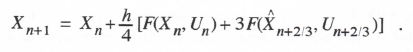
(3.170)

Here the first-pass estimate for is based on the area from t = nh to t = (n+1/3)h under a quadratic approximation for F(t) which passes through F_n, F_n-1 and F_n-2. The second-pass estimate for X_n+2/3 is based on the area from t = nh to t = (n+2/3)h under a quadratic approximation for F(t) which passes through F_{n+ 1/3}, F_n and F_n-1. The final pass for X_n+1 is based on the area from t = nh to t = (n+1)h under a quadratic approximation for F(t) which passes through F_n+2/3, F_n+1/3 and F_n. For this real-time three-pass predictor-corrector algorithm the integrator error coefficient e_I = 1/216 and the algorithm order k = 3. Since the first two passes have local truncation errors proportional to h⁴, this third-order algorithm exhibits global asymptotic errors of order h³ which are the same as those for a single-pass method based on mechanizing Eq. (3.170) when F = U. Thus all of the formulas in Section 3.3 for characteristic root errors and transfer function gain and phase errors will apply, with e_I= 1/216 and k = 3. Note that the method is compatible with real-time inputs, since U_n is required at the beginning of the first pass, U_n+1/3 at the beginning of the second pass, and U_n+2/3 at the beginning of the third pass.

It is useful to compare the above integration method with RK-3 integration as given in Eqs. (1.35), (1.36) and (1.37). There is computed in the first two passes using the RTRK-2 algorithm given in Eqs. (1.27) and (1.28), but with a step size of 2h/3 rather than h. The formula in Eq. (1.37) for the final pass which computes X_n+1 is the same as Eq. (3.170) above. For RK-3 integration we have seen in Eq. (3.117) that the fractional error in characteristic root is given by . For the three-pass algorithm represented by Eqs. (3.168), (3.169) and (3.170) with e_I = 1/216, it follows from Eq. (3.45) that . Thus the RK-3 root error is a factor of nine larger. The increased characteristic root error for RK-3 integration results from the larger error associated with the use of the second-order RTRK-2 method rather than the third-order predictor-corrector method in the computation of .

An interesting variation of the three-pass method of Eqs. (3.168), (3.160) and (3.170) is to use a second-order rather than third-order predictor formula for computing in the first pass. In this case the formulas become

(3.171)

(3.172)

(3.173)

Here the integrator error coefficient is still given by , since a third-order predictor formula is used to compute in the second pass.

To determine the stability regions in the λh plane for the above three-pass predictor-corrector methods we apply the algorithms to the first-order system with transfer function H(s) = 1/(s – λ), as given by Eq. (3.1). By rewriting the resulting difference equations with a step size T = h/3 and taking the Z transform, we can solve for H*(z) = X*(z)/U*(z). As before, from the denominator of H*(z) we can determine the stability boundary in the λh plane for each of the two algorithms by calculating λh for values of z on the unit circle in the z plane. The results are shown

3-49

in Figure 3.12, along with the stability boundary obtained previously for RK-3 integration. Also shown in the figure for comparison purposes is the stability boundary for AB-3 integration, which has been multiplied by three to take into account the fact that it is a single-pass method which executes three times faster than the three-pass methods. Figure 3.12 shows that the overall stability region for RK-3 integration is the largest, with P-2/PC-3/C-3, the abbreviation used for the method given by Eqs. (3.171), (3.172) and (3.173), the next largest. The boundary for P-3/PC-3/C-3, which is the abbreviation used for the method of Eqs. (3.168), (3.169) and (3.170), is the next largest. The AB-3 stability boundary, even after normalization with a factor of three gain, exhibits the smallest overall size.

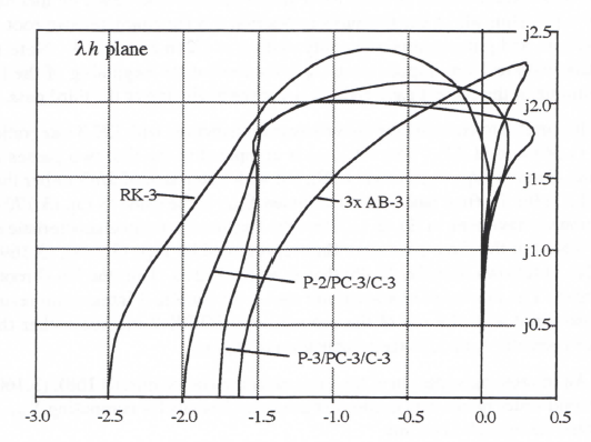
Figure 3.12. Stability boundaries for three-pass integration methods and AB-3

integration, normalized.

Thus the price paid for the factor of nine improved accuracy over RK-3 integration for the three-pass predictor-corrector methods introduced in this section is a somewhat reduced stability region. To compare the accuracy of the methods with AB-3 integration, we must take into account the fact that AB-3, as a single-pass method, executes approximately three times as fast. Thus the error coefficient , e_I= 1/216, for the three-pass methods should be increased by a factor of 3³ or 27 for a direct comparison with AB-3 integration. When this is done, the resulting normalized integrator error coefficient e_I = 27/216 = 1/8, compared with e_I = 3/8 for AB-3 integration. Thus the three-pass predictor-corrector methods have a factor of three accuracy advantage over AB-3 integration, in addition to enjoying a slight stability edge.

3-50

3.12 Accuracy of the Asymptotic Formulas for Dynamic Errors

The asymptotic formulas derived in this chapter for the dynamic errors associated with integration algorithms are only valid when the integration step size h is sufficiently small (|λh| << 1 for characteristic root errors, ωh << 1 for transfer function errors). For the different integration methods considered here, Table 3.1 summarizes the formulas for the approximate fractional errors

Table 3.1

Summary of Asymptotic Formulas for Characteristic Root Errors

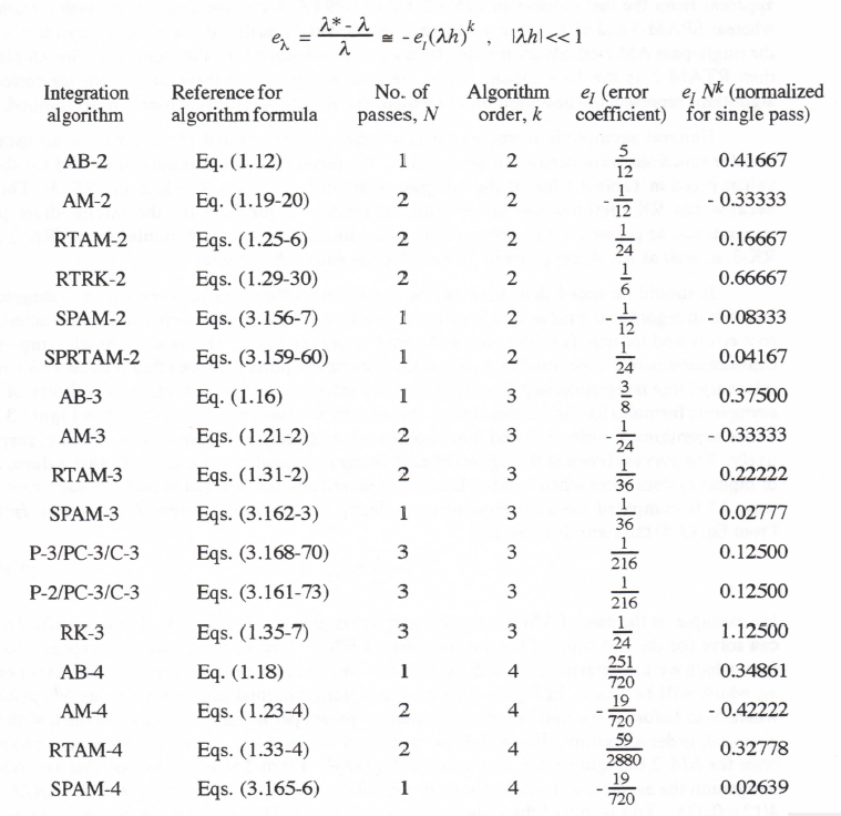
3-51

in the characteristic roots. In the last column of the table the integrator error coefficient, e_I, has been normalized through multiplication by N^k, where N is the number of passes (state-variable derivative calculations) associated with the given integration algorithm. For example, N =2 and k = 2 for AM-2 integration, since it is a two-pass algorithm of second order. This means that in general it will require twice as long to execute as the single-pass AB-2 method, which in turn means that the mathematical step size h in a real-time simulation will need to be twice as large. Since the root error is proportional to h^k, i.e., h² in this case, the error will be 2² = 4 times larger than it would be for a single-pass algorithm with the same e_I . Thus among algorithms of the same order the normalized error coefficient is a true indication of the relative accuracy of each method for small step size (|λh|<< 1). Based on asymptotic errors in the characteristic root, then, it is apparent from the last column in Table 3.1 that SPRTAM-2 is the best second-order method, whereas SPAM-3 and SPAM-4 represent the best third and fourth-order methods, respectively. If the single-pass AM methods are rejected because of their reduced stability regions in the Ah plane, then RTAM-2 is the best second-order method, either of the three-pass predictor-corrector algorithms represent the best third-order method, and RTAM-4 is the best fourth-order method.

General asymptotic formulas for fractional gain errors and phase errors in sinusoidal transfer functions were derived in Section 3.3. We recall that these formulas are valid for the e_I values listed in Table 3.1 for all the integration algorithms except RTRK-2 and RK-3. This is because the RK methods use lower-order integration algorithms for the intermediate-pass integrations, as pointed out in Section 3.6. The gain and phase error formulas for RTRK-2 and RK-3, as well as RK-4, are given in Table 3.2 at the end of this chapter.

It should be noted that there can be significant differences between various integration methods in regard to the range of |λh| or ωh over which the asymptotic formulas for characteristic root errors and transfer function gain and phase errors are valid. This is an especially important consideration in real-time simulation, where the accuracy requirements are often modest and where relatively large integration step sizes are therefore often used. The |λh| range of validity of the asymptotic formulas for the fractional error in characteristic root, e_|λ|, is illustrated in Figure 3.13, where algorithms of order 2, 3 and 4 are compared separately in Figures 3.13a, b and c, respectively. The curves shown in the figure for each integration method are based on exact values, λ*, of digital system roots when solving Eq. (3.1) numerically for λ negative real. In each case the exact λ* is computed from the appropriate pole, z₁ , of the digital system Z transform, H*(z). From Eq. (3.5) the formula is simply

(3.174)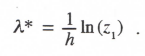

For example, in the case of AM-2 integration, H*(z) is given by Eq. (3.134). For a specific λh we can solve for the two roots of the denominator of H*(z). One of these roots corresponds to z₁, from which we can determine λ* with Eq. (3.174). We can then determine the fractional root error e_λ, which will be exact. In Figure 3.13 we have plotted normalized root errors as N^ke_λ/(λh)^k, where N as before is the number of state-equation passes per integration step associated with the given kth-order algorithm. For AM-2 integration, N = 2 and k = 2. Hence the normalized root error for AM-2 in Figure 3.13a is plotted as 4e_λ/(λh)². From Table 3.1 we see that for AM-2 integration the asymptotic formula for e_λ is –e_I(λh)² = (λh)²/12. Thus N^ke_λ/|λh|k = 4e_λ/(λh)² = 4/12 = 0.333. This is indeed the value for the normalized AM-2 root error in Figure 3.13a when

3-52

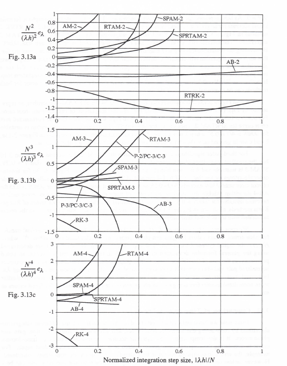
Figure 3.13. Normalized characteristic root errors for 2nd, 3rd and 4th-order integration methods.

3-53

|λh| = 0. As |λh| increases, the normalized error increases. This is because the asymptotic formula is less accurate for larger |λh| values. N is also equal to 2 for the two-pass RTAM-2 and RTRK-2 methods in Figure 3.13a, whereas N = 1 for the single-pass AB-2, SPAM-2 and SPRTAM-2 algorithms. The abscissa in Figures 3.13a, b and c is the normalized integration step size, |λh|/N. By dividing the dimensionless step size magnitude |λh| by N, we have taken into account the fact that an N-pass algorithm will require a mathematical step size N times larger than a single-pass algorithm. For example, if λh = 0.2 for a single-pass method, then we must let λh = 0.4 for a two-pass method (N =2) to obtain the same processor execution time per overall integration step. In both cases |λh|/N = 0.2 in Figure 3.13. Thus the normalized characteristic root error for both methods can be compared at the same abscissa value.

From Figure 3.13a it is apparent that for |λh|/N < 0.54 the SPRTAM-2 algorithm, as represented by Eqs. (3.159) and (3.160), exhibits the smallest magnitude of characteristic-root error. For |λh|/N > 0.54, AB-2 has the smallest root error in Figure 3.13a. Note that the normalized root error curve for SPRTAM-2 is not shown for |λh| > 0.57. This is because the algorithm is unstable for |λh|/N > 4/7 0.57 when λ is negative. In fact the normalized root error plots in Figure 3.13a, b and c are in general only shown for |λh|/N values for which each algorithm is stable.

For third-order algorithms Figure 3.13b shows that the SPAM-3 method of Section 3.10 has the smallest magnitude of characteristic root error for |λh|/N < 0.29. For |λh|/N > 0.29, SPAM-3 is unstable and AB-3 exhibits the smallest root errors. From Figure 3.13c for fourth-order algorithms we see that the SPAM-4 method of Section 3.10 exhibits the smallest magnitude of root error until |λh|/N exceeds 3/190.15, beyond which it goes unstable. For |λh|/N > 0.15 the AB-4 algorithm exhibits the smallest magnitude of normalized characteristic root error until it becomes unstable for |λh|/N > 0.3. Note that the normalized characteristic root errors of Runge-Kutta methods, as shown in Figure 3.13a, b and c, are in every case much larger than the errors associated with the best real-time methods.

We consider next the ωh range of validity of the asymptotic formulas for sinusoidal transfer function errors. Exact values for gain and phase errors can be calculated from H*(e^jωh), where H*(z) is the digital system Z transform. The approximate formulas for ωh << 1 are determined using the general formulas developed in Section 3.3 in terms of e_I and k except, as noted previously, in the case of the RK methods. Here a graphical comparison of exact and approximate normalized gain and phase errors is more complicated, since the errors depend on both ωh and λh. In general, however, the trends evident in Figure 3.13 for characteristic root errors are similar when normalized transfer function gain and phase errors are plotted versus λh for fixed values of ωh.

3.13 Comparison of Time-domain Errors

Until now we have only compared the dynamic accuracy of the different integration algorithms by considering characteristic root errors, and sinusoidal transfer function gain and phase errors. It is also tempting to make dynamic accuracy comparisons based on time-domain errors in simulating the response of a given system to a specific time-dependent input. For example, the errors in computed response to a step-function input are sometimes considered. However, unless one is specifically interested in step-function response accuracy, this can be a very misleading method for dynamic accuracy comparison in the case of integration algorithms which employ predictor methods. This is because predictor algorithms of order two and higher will have large transient errors introduced by the step input. The accuracy of predictor methods depends on the existence of input derivatives, a condition which is violated by a step function input. In fact, the dynamic accuracy of the time-domain response is often completely dominated by the startup transient generated as a result of a step input.

In an attempt to avoid this difficulty we will consider in this section the errors of the various integration methods in simulating the response of a dynamic system to a step displacement input with limited acceleration. For simplicity we let the dynamic system be represented by the following second-order linear system:

(3.175)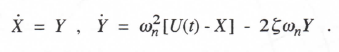

Here X is the output, U(t) is the input, ω_n, is the undamped natural frequency, and ζ is the damping ratio. We let U(t) be an acceleration-limited unit step function given by

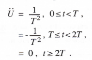
(3.176)

When integrated twice with T set equal to 1.2/ω_n, Eq. (3.176) yields the input U(t) shown in Figure 3.14. The second-order linear system response to this input with initial conditions X(0) = Y(0) = 0 is also shown in the figure. For comparison purposes the response to a true unit step input applied at t = T, i.e., at ω_nt = 1.2, is shown as the dashed curve in Figure 3.14. Since the ideal unit step response is quite similar, it is apparent that the use of the acceleration-limited step input, which eliminates input discontinuities in displacement and slope, does not in fact change appreciably the shape of the second-order system step response. In actuality the acceleration-limited step input is probably a more realistic input for a mechanical dynamic system.

We consider first the performance of second-order integration algorithms. We have already noted that some of the traditional second-order integration methods are not compatible with real-time inputs. For example, AM-2 is a two-pass method that requires the input U_n+1 at the beginning of the second (i.e., corrector) pass, halfway through the nth integration frame and therefore half a frame before it is available in real time. However, at the end of the first (i.e., predictor) pass, the estimate, _n+1, has been computed and is available as a real-time output. Although the accuracy of _n+1 will in general be less than the accuracy of X_n+1, the error in _n+1 will be a local truncation error, proportional to h³. In Figure 3.15 we have plotted both the error in X_n, and the estimate _n, versus dimensionless time ω_nt when AM-2 is used to compute the second-order system response to the acceleration-limited step input. The integration step size is given by ω_nh = 0.2 and the initial conditions are taken as X₀ = Y₀ = X_-1 = Y_-1 = 0, which solves the second-order predictor startup problem. From the figure it is apparent that the errors in X_n , and _n are quite comparable. Therefore, in this example at least, little if any accuracy is lost by considering _n as the real-time output. Thus _n will be used hereafter as the AM-2 output in all subsequent accuracy comparisons with other integration methods.

In the case of RTAM-2 we have seen that the algorithm is compatible with real-time inputs, since at the start of the first pass the input U_n is required and at the start of the second pass, U_n+1/2

3-55

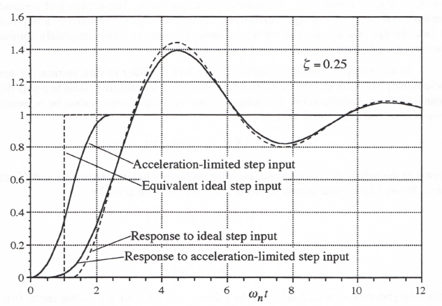
Figure 3.14. Response of second-order system to an acceleration-limited unit-step input.

 

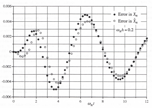
Figure 3.15. AM-2 step response errors for both predictor and corrector passes.

3-56

is required, both of which are available in real time. Actually, the half-frame predictor estimate, _{n+ 1/2}, is quite comparable in accuracy to that of the final corrector output X_n+1 at the end of the nth frame. This is evident in Figure 3.16, where the errors at both half-integer and integer frame times are shown for the case where RTAM-2 is used to simulate the second-order system with the acceleration-limited step input. As in the previous AM-2 solution, the simulation is started with X₀ = Y₀ = X_-1 = Y_-1 = 0 and ω_nh = 0.2. The results in Figure 3.16 suggest that in general both X_n and _n+1/2 can be employed as outputs when RTAM-2 integration is used. Thus the method generates real-time outputs at twice the basic integration frame rate, 1/h. Comparison of the errors in Figures 3.15 and 3.16 shows that RTAM-2 is approximately twice as accurate as AM-2. This is expected, since the integrator error coefficient e_I = 1/24 for RTAM-2 and -1/12 for AM-2.

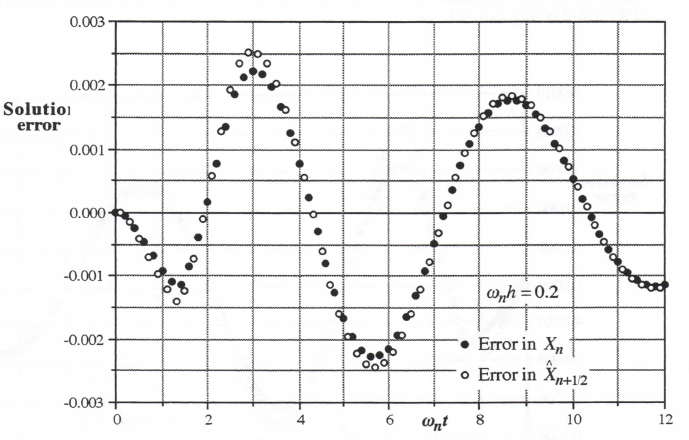
Figure 3.16. RTAM-2 step response error for both predictor and corrector passes.

In Section 3.10 we noted that the single-pass version of RTAM-2, denoted as SPRTAM-2, produces an nth-frame output, X_n+1 , which is not strictly compatible with real time. This is because the input U_{n+ 1/2} is required in Eq. (3.160) at the start of the nth frame, unless calculations involving U_n+1/2 can be postponed until at least halfway through the frame. Again, however, we can consider use of the estimate _n+1/2, as a real-time output. This is because the computation of _n+1/2 using Eq. (3.159) can be initiated halfway through the previous frame, at t = (n – 112)h, and can therefore be completed at t = (n – 1/2)h, as required in real time. In Figure 3.17 the errors in both _n+1/2 and X_n are shown for the case where SPRTAM-2 is used to simulate the second-order system with the acceleration-limited step input. Initially the simulation is started with X₀ = Y₀ = X_-1/2 = Y_-1/2 = X_-3/2 = Y_-3/2 = 0, which would be the case if the second-order system had been in equilibrium with zero input for t < 0. Here we let the integration step size be given by ω_nh = 0.1 instead of 0.2, since the single-pass algorithm will execute twice as fast per integration step as the two-pass AM-2 and RTAM-2 algorithms. The results in Figure 3.17 show that _n+1/2 can be employed as a real-time output when SPRTAM-2 integration is used without any appreciable loss in accuracy, at least in the example considered here. Thus the half-integer output, _{n+ 1/2}, is generated in real time and the integer output, X_n, is generated half a frame behind real time when using SPRTAM-2. However, if the computational order within each frame can be rearranged so that U_n+1/2 is not needed until halfway through the frame, then both X_n and _n+1/2 can be made available as real-time outputs when using SPRTAM-2. Comparison of Figure 3.17 with Figure 3.16 shows that the SPRTAM-2 errors are roughly one quarter the RTAM-2 errors. This is as expected, since the integrator error coefficient e_I = 1/24 for both methods and the step size for SPRTAM-2 is only half as large.

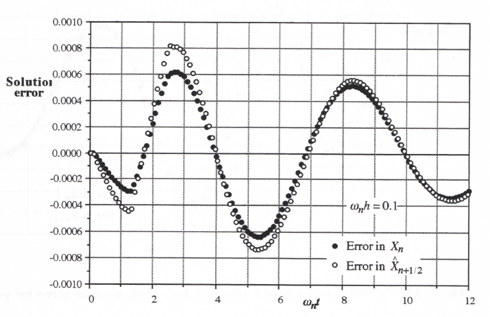
Figure 3.17. SPRTAM-2 step response error for both integer and half-integer frame outputs.

In Figure 3.18 the response errors for RTRK-2, AB-2, AM-2, RTAM-2, and SPRTAM-2 are all plotted versus ω_nt. Initial conditions on X and Y are assumed to be zero for t ≤ 0. The integration step size ω_nh = 0.1 for the single-pass AB-2 and SPRTAM-2 methods, and 0.2 for the two-pass RTRK-2, AM-2 and RTAM-2 methods. As noted earlier, this is because single-pass methods will execute approximately twice as fast as two-pass methods on a given processor. In the case of AM-2 the errors are shown for the predicted output, , in order to be representative of a real-time output, as noted above. Similarly, in the case of SPRTAM-2 the errors are shown for the half-integer frame output, , again to be representative of a real-time output. The results in Figure 3.18 show that the SPRTAM-2 predictor-corrector method introduced in Section 3.10 is the most accurate, as measured by the response errors here for an acceleration-limited step input. The next most accurate method is RTAM-2. This is just what we would have predicted for second-order integration methods based on the normalized integrator error coefficients in Table 3.1 and in Figure 3.13

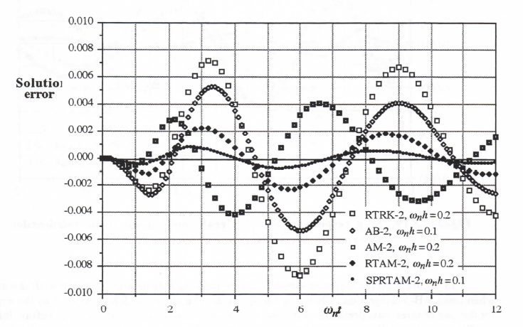
Figure 3.18. Step response errors for real-time outputs using second-order integration methods.

We consider next the performance of third-order integration methods. The response errors for AB-3, AM-3, RTAM-3, and SPAM-3 are plotted versus in Figure 3.19. Again, initial conditions on X and Y are assumed to be zero for . Thus X₀ = Y₀ = X_-1 = Y_-1 = X_-2 = Y_-2 = 0, which solves the third-order predictor startup problem. The integration step size = 0.1 for the single-pass AB-3 and SPAM-3 methods, and 0.2 for the two-pass AM-3 and RTAM-3 methods. In the case of both AM-3 and SPAM-3 the errors are shown for the predicted output, , in order to be representative of a real-time output, as noted above for AM-2. The results in Figure 3.19 show that the SPAM-3 method is the most accurate, as measured by the response errors for an acceleration-limited step input to a second-order system. The next most accurate method is RTAM-3, followed by AB-3 and AM-3. Again, this is consistent with the normalized integrator error coefficients in Table 3.1 and in Figure 3.13 for third-order integration methods.

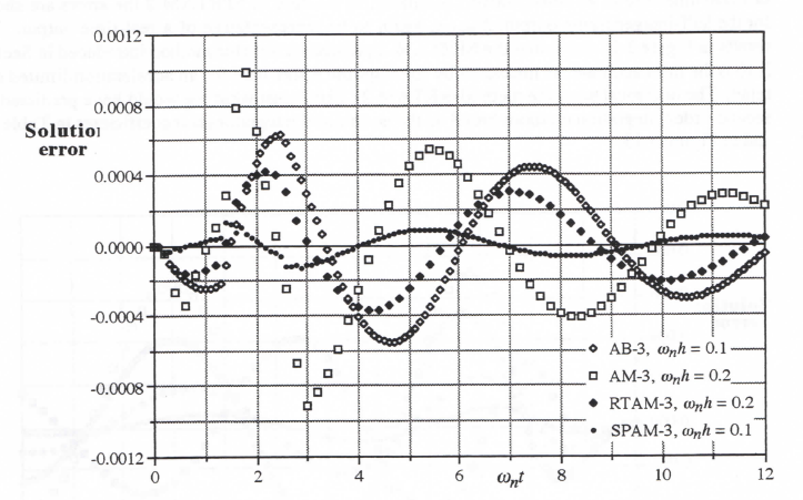
Figure 3.19. Step response errors for real-time outputs using third-order integration methods.

In Figure 3.20 the response errors for three-pass algorithms are compared with the error when using AB-3 integration. Shown in the figure are the errors for RK-3, as well as the errors for the pair of three-pass predictor-corrector methods introduced in Section 3.11. As before, initial conditions on X and Y are assumed to be zero for . The integration step size = 0.1 for the single-pass AB-3 method, and 0.3 for the three-pass RK-3, P-3/PC-3/C-3 and P-2/PC-3/C-3 methods. The results in Figure 3.20 show that RK-3 is the least accurate method by a fairly wide margin. The most accurate is the P-3/PC-3/C-3 algorithm, followed by P-2/PC-3/C-3 and AB-3. Comparison of Figures 3.19 and 3.20 shows that the SPAM-3 algorithm is the most accurate of all the third-order algorithms considered here, at least based on simulating the example second-order system with an acceleration-limited unit step input. The three-pass predictor-corrector-method, P-3/PC-31C-3 as given by Eqs. (3.168-70), is the next most accurate and may be preferred over SPAM-3 when stability is of concern. This is evident by comparing Figures 3.11 and 3.12, even when the stability boundary for SPAM-3 is multiplied by 3 because it executes three times as fast. Note that all of the three-pass methods provide estimates in the nth frame for and as well as the final . In the case of P-3/PC-3/C-3 these intermediate estimates have local truncation errors proportional to h⁴ and can be used to provide accurate real-time outputs one-third and two-thirds the way through each frame. In the case of P-2/PC-3/C-3, which uses second-order prediction for the first pass, the local truncation error in is proportional to h³ and will therefore be less accurate. The second pass in P-2/PC-3/C-3 does use a third-order corrector and hence produces a local truncation error in proportional to h⁴. In the case of RK-3, which uses simple Euler integration for the first pass, the local truncation error in is proportional to h² and will be even less accurate. The second RK-3 pass uses RTRK-2, with the local truncation error proportional to h³. Thus the RK-3 estimates one-third and two-thirds the way through each frame will be considerably less accurate than the intermediate P-3/PC-3/C-3 outputs.

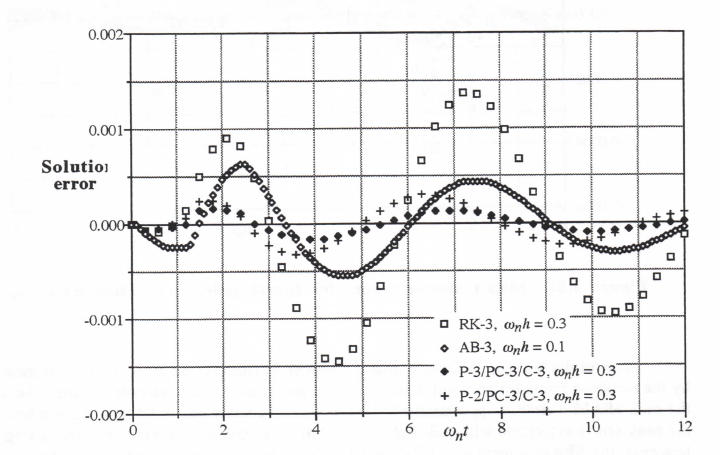
Figure 3.2. Step response errors for three-pass third-order integration methods.

Finally, we consider the time-domain errors when fourth-order integration algorithms are used to simulate the second-order system with an acceleration-limited unit step input. The results for AB-4, AM-4, RTAM-4, and SPAM-4 are plotted versus in Figure 3.21. Also shown for comparison purposes is the result when RK-4 integration is used, even though RK-4 is not compatible with real-time inputs. As before, initial conditions on X and Y are assumed to be zero for . Thus X₀ = Y₀ = X₊₁ = Y_-1 = X _-2 = Y_-2 = X_-3 = Y_-3 = 0. The integration step size = 0.1 for the single-pass AB-4 and SPAM-4 methods, 0.2 for the two-pass AM-4 and RTAM-4 methods, and 0.4 for the four-pass RK-4 method. In the case of both AM-4 and SPAM-4 integration, the errors are shown for the predicted output, , in order to be representative of a real-time output.

3-61

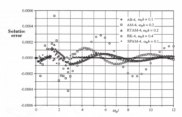
Figure 3.21. Step response errors for fourth-order integration methods.

The results in Figure 3.21 show that the SPAM-4 method is the most accurate, as measured by the response errors for an acceleration-limited step input to a second-order system. Actually, the peak SPAM-4 error of approximately 0.0001, which occurs at = 1.4, is not much less than the peak errors associated with AB-4 and RTAM-4. Once the startup transient errors damp out, however, the SPAM-4 method exhibits much smaller errors. The relatively large startup error associated with the SPAM-4 method occurs despite the acceleration limiting in the unit step input. This is because the input, as shown in Figure 3.14, does have discontinuities in its second time derivative at = 0, 1.2, and 2.4. These discontinuities generate large transient errors in the third-order predictor algorithms. Once the input discontinuities no longer occur, the SPAM-4 errors become very small indeed compared with the other fourth-order methods. In the case of AB-4, the other single pass method of Figure 3.21, this is because the integrator error coefficient for SPAM-4 is 19/720, compared with 251/720 for AB-4 (see Table 3.1). In comparison with the two-pass AM-4 and RTAM-4 methods, the single-pass SPAM-4 executes twice as fast and hence gains a factor of 16 in accuracy because of the error dependance on h⁴. Since SPAM-4 executes four times as fast as the four-pass RK-4 method, it gains a factor of 4⁴ or 256 in accuracy. This more than offsets the much smaller error coefficient associated with RK-4 for a given step size h. It should also be noted again that the errors plotted in the figure for AM-4 are based on the estimated or predicted output value, , rather than the corrected value, X_n+1. It turns out for AM-4 that the initial peak error associated with X_n+1 is only about one-fifth the initial peak error associated with although the AM-4 errors for X_n+1 and become quite comparable after the effects of the input discontinuities die out.

3-62

3.14 Accuracy Summary for Real-time Integration Methods

In this chapter we have examined the accuracy of integration algorithms suitable for real-time simulation of dynamic systems, including algorithms of order one through four. Dynamic errors have been analyzed by considering linearized versions of the nonlinear differential equations used to model the system being simulated. For each of the real-time integration methods we have developed in the frequency domain an approximate model of the numerical integrator. This model takes the form of an integrator transfer function for sinusoidal inputs, as shown in Eq. (3.37). In terms of the integrator error coefficient e_I and order k for each algorithm we have been able to develop approximate formulas for the characteristic root errors, as well as the transfer function gain and phase errors, in simulating the linearized version of dynamic systems. These approximate formulas provide good indicators of the dynamic accuracy to be expected for a given step size h in simulating nonlinear systems.

The first-order Euler integration algorithm, with dynamic errors proportional to the integration step size h, is the least accurate method. It should be used only when high dynamic accuracy is not required and the step size h is small compared with the shortest time constants prevalent in the simulation. The AB-2, AB-3 and AB-4 predictor algorithms are single-pass methods (one evaluation of each state-variable derivative per integration step) which are both popular and suitable as real-time integration methods. The higher order AB algorithms can exhibit stability problems, as is evident in the -plane stability boundaries shown in Figure 3.2. The AM-2, AM-3 and AM-4 predictor-corrector algorithms are two-pass methods which are not compatible with real-time inputs U, since they require the input U_n+1 during the nth integration frame, before it is available in real time. However, if the predicted output, , is used instead of the final corrected output, X_n+1, the AM methods can be made real-time compatible, as we showed in the time-domain results just completed in Section 3.13. On the other hand, we have demonstrated that two-pass real-time versions of the AM predictor methods, namely RTAM-2, 3 and 4, produce two outputs, X_n+1/2 and X_n+1, per integration frame and have complete compatibility with real-time inputs. Also, the RTAM methods exhibit better accuracy and stability performance than AM methods. We have also introduced single-pass versions of the predictor-corrector methods, designated as SPAM and SPRTAM. In these algorithms only the derivatives based on the predicted states are used, which means that they execute twice as fast as the two-pass predictor-corrector methods. This in turn means for small step size h that they produce dynamic errors equal to 1/4, 1/8, and 1/16 the errors for the two-pass methods of order 2, 3, and 4, respectively. Thus they represent potentially the most accurate of all the algorithms considered here, as shown by the normalized integrator error coefficients presented in Table 3.1 on page 84 and the time-domain results in the section just completed. The SPAM and SPRTAM algorithms do suffer from very limited stability regions in the -plane and may therefore be unsuitable in many real-time applications.

The Runge-Kutta methods considered in this chapter are generally not competitive in accuracy with the above integration algorithms, although the RTRK-2 and the RK-3 methods are compatible with real-time inputs. In Section 3.11 we introduced a pair of three-pass predictor-corrector methods which significantly outperform RK-3 and even the single-pass predictor-corrector method when the step size h lies outside the SPAM-3 stability boundary in the plane. Also, the general formulas for transfer function gain and phase errors, as derived in Section 3.3 in terms of the integrator error coefficient, e_I, are not applicable to Runge-Kutta methods. Table 3.2 at the end of this chapter lists the asymptotic formulas for transfer-function gain and phase errors for RK-2, RTRK-2, RK-3 and RK-4.

In Section 3.12 we noted that there can be significant differences between various integration methods in regard to the range of or over which the asymptotic formulas for characteristic root errors, and transfer function gain and phase errors, are valid. This is an especially important consideration in real-time simulation, where the accuracy requirements are often modest and where relatively large integration step sizes are therefore frequently used. The range of validity of the asymptotic formulas for the fractional error in characteristic root, , is illustrated in Figure 3.13 by plotting the exact errors versus normalized integration step size.

3-64

Table 3.2

Runge-Kutta Characteristic Root and Transfer Function Errors

3-65

3-66