The method of Z transforms was originally developed for analysis of sampled-data control systems, i.e., dynamic systems utilizing a mixture of continuous and discrete time signals. This is just the case, for example, when a digital computer is used to control a continuous process. The Z transform method is equally valuable in analyzing all-digital systems, and in particular for the determination of dynamic errors in digital simulation. The dynamic errors will depend on the type of numerical integration algorithm and the integration step size. The method of Z transforms permits us to examine these errors analytically and hence choose acceptable integration algorithms and steps sizes to meet prescribed accuracy requirements. The method is restricted to linear systems with a fixed time step or sample period. We have already noted in Chapter 1 that nonlinear systems, for purposes of dynamic error analysis, can usually be linearized using perturbation equations, and that real-time digital simulations traditionally employ fixed integration step sizes. Thus the Z transform requirements can be met.
2.2 Definition of the Z Transform
We will assume that the digital signals involved in digital simulation are data sequences, with the individual numbers in each data sequence considered to be equally spaced in time, as noted above. Thus the digital signal or data sequence representing a continuous time function f(t) will be denoted as the data sequence {fn} where each individual data points fn represents f(nh)with n = 0, 1, 2, … . Here h is the time interval between successive numbers in the data sequence. In the digital simulation of a continuous dynamic system h is the integration step size.
The Z transform of the digital data sequence {fn} is defined as

 (2.1)
(2.1)
where z is a complex variable. We note the similarity of the Z-transform definition to the definition of the Laplace transform of a continuous time function f(t).* Thus

 (2.2)
(2.2)
The integral of the continuous time function in the Laplace transform is replaced by the summation of the discrete time series in the Z transform. For data sequences derived from exponential time functions, the Z transform can be written in closed form. Consider the exponential time function
![]()
![]() (2.3)
(2.3)
and the equivalent data sequence

 (2.4)
(2.4)
where
![]()
![]() (2.5)
(2.5)
From Eq. (2.1) we see that

 (2.6)
(2.6)
Expansion of (1 – Az-1)-1 using the binomial theorem easily proves the validity of Eq. (2.6). Thus we have shown that
![]()
![]() (2.7)
(2.7)
It also follows that if the Z transform of a data sequence contains a term z/(z – A), the corresponding data sequence is the exponential sequence, {eonh}, i.e., equivalent to equally spaced samples from a continuous time function eotwith a sample interval h. From Eq. (2.5)
![]()
![]() (2.8)
(2.8)
It is useful to consider the case of a complex exponential function
![]()
![]() (2.9)
(2.9)
We recall that together with the conjugate function e(σ–jw)t this can be used to represent a sinusoidal time function of frequency ω with an exponentially varying amplitude eot. Here the equivalent data sequence is
![]()
![]() (2.10)
(2.10)
where A is now complex and is given by
![]()
![]() (2.11)
(2.11)
But the complex number A can be written as

(2.12)
where

 (2.13)
Equating the right sides of Eqs. (2.11) and (2.12), we have

 (2.14)
Thus a Z transform given by z/(z–A), where A is complex, corresponds to a data sequence derived from equally-spaced samples of a sinusoidal time function of frequency ω and amplitude eot. The formulas in Eq. (2.14) relate ω and σ to the complex constant A. We note from both Eq. (2.8) for A positive real and Eq. (2.14) for A complex that the data sequence amplitude decreases exponentially for |A| < 1 and increases exponentially for |A| > 1. For A = 1 the data sequence is always unity, i.e., fn = 1 for all n. For A = -1 the data sequence alternates, i.e., f0 = +1, f1 = -1, f2= +1, f3 = -1 etc., which represents samples from a unit amplitude sinusoid with frequency equal to one-half the sample frequency, as predicted by Eq. (2.14). Thus ω = π/h for A = -1 and hence the sinusoidal period = 2π/ω=2h.
2.3 Simple Example of a Linear Digital System
We have seen in the previous section how the Z transform can be used to represent a data sequence. In this section we will see how the Z transform can be used to represent a digital system. As a simple example, consider the continuous first-order linear system shown in Figure 2.1 and described by the differential equation
![]()
![]() (2.15)
(2.15)

 Figure 2.1. First-order continuous system.
Assume that we wish to simulate this system digitally using Euler integration. In Chapter 1 we have seen that the numerical solution of Eq. (2.15) with Euler integration leads to the following difference equation:
![]()
![]() (2.16)
(2.16)
This is the difference equation mechanized by the digital simulation, starting at t = 0 (i.e.,n = 0) with x0 as the initial condition. The equation is now iterated for n = 0, 1, 2, … ,to produce the outputs x1, x2, x3, … , in response to the inputs f0, f1, f2, f3, … . Thus the digital computer produces an output data sequence {xn+1} given from Eq. (2.16) by
![]()
![]() (2.17)
(2.17)
where {fn} is the input data sequence. We now take the Z transform of the data sequences appearing on both sides of Eq. (2.17). Consider first the Z transform of {xn+1} From Eq. (2.1) this is given by

or
![]()
![]() (2.18)
(2.18)
Note the similarity of Eq. (2.18) to the formula for the Laplace transform of the derivative of a function. Thus
![]()
![]() (2.19)
(2.19)
Using Eq. (2.18), we can now take the Z transform of Eq. (2.17) and obtain
![]()
![]() (2.20)
(2.20)
Solving for X*(z) we have

 (2.21)
The first term on the right side of Eq. (2.21) depends only on the initial condition x0 and is equivalent to the transient (complementary) solution in the case of a continuous system. It has exactly the form of Eq. (2.7) and therefore represents in the time domain an exponential data sequence x0{(eoh)n} = x0{A}n , where A = 1 + λh. From Eq. (2.8) we see that
![]()
![]() (2.22)
(2.22)
We note that 1n (1 + y) = y –y2/2 + y3/3 – y4/4 + ∙∙∙ , . Expanding the 1n function in Eq. (2.22), we have

or

 (2.23)
For the continuous linear system the transient solution is given by x0eλ1, so that a “perfect” digital solution would be the data sequence x0{(eλh)n}, compared with our actual solution, x0{(eoh)n}. Just as λ is the characteristic root of the continuous system, so is σ the equivalent characteristic root of the digital system. From now on we will designate the characteristic root of the digital system by λ*, where λ* = σ in our example here. Replacing σ with λ* in Eq. (2.23), subtracting λ and dividing by λ, we obtain the following formula for eλ, the fractional error in the characteristic root of our digital system:

 (2.24)
The above asymptotic formula is valid only for h<<1/|λ|. But this will of necessity be true if we are to have an accurate simulation. As expected for Euler integration, the root error varies as the first power of the integration step size h. Thus the root error will decrease by a factor of two whenever we halve the step size.
We next consider the second term on the right side of Eq. (2.21), i.e., the term involving the input Z transform, F*(z). The coefficient of F*(z) in this term is defined as the Z transform, H*(z), of the digital system. Thus

 (2.25)
and when x0 = 0,
![]()
(2.26)
Thus the system Z transform, H*(z), times the input Z transform, F*(z), yields the output Z transform, X *(z), as shown in Figure 2.2. The analogy with the Laplace transform representation of the continuous system, as shown in Figure 2.1b, is very evident.
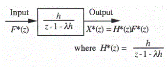
Figure 2.2. Digital system representing simulation of a first-order system using Euler integration.
Using Euler integration, we now compute the response of our first-order linear system to a unit data point input defined by
![]()
![]() (2.27)
(2.27)
Iterating the difference equation (2.16) with zero initial condition (x0 = 0), we obtain
![]()
![]() (2.28)
(2.28)
It turns out that we can get also obtain the unit data point response of our digital system directly from the system Ztransform, H*(z), given in Eq. (2.25). To do this we divide the denominator into the numerator of H*(z) to create a power series in z-1, as shown below.
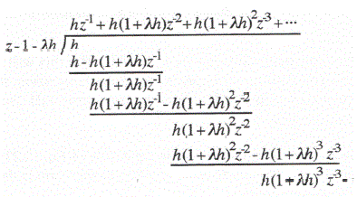
Thus
![]()
![]() (2.29)
(2.29)
From the Z-transform definition in Eq. (2.1) we see that the data sequence {wn} for which H*(z) is the Z transform is given by
![]()
![]() (2.30)
(2.30)
I.e., when the Z transform is expressed as a series in powers of z-1, the coefficient of z–n is wn, the data sequence value at time nh. The data sequence represented by Eq. (2.30) is identical with the data sequence obtained in Eq. (2.28) in response to a unit data point input. We conclude that the time-domain representation of the Z transform, H*(z), of a digital system is simply the unit data point response, {wn}, of the digital system. Conversely, the Z transform of the unit data point response is the system Z transform, H*(z). This also follows if we consider the Z transform of the unit data point input represented by Eq. (2.27). From Eq. (2.1) the corresponding Z transform is simply F*(z) = 1. When F*(z) = 1 we conclude from Eq. (2.26) that X*(z) = H*(z), i.e., the Z transform of the unit data point response is indeed the system Z transform.
The unit data point input to a digital system is analogous to a unit impulse input, δ(t)for a continuous system. The response data sequence, {wn} of the digital system is analogous to the unit-impulse response, W(t), of the continuous system. Just as the Z transform of the unit data point response data sequence, {wn}, is H*(z), the system Z transform, in the case of a continuous system the Laplace transform of the unit impulse response, W(t), is the Laplace transform (transfer function), H(s), of the continuous system.
It is useful to write Eq. (2.26) with the Z transforms expressed in series form. Thus

 (2.31)
Equating coefficients of like powers of on both sides of Eq. (2.31), we obtain

 (2.32)
Since fn-k = 0 for k > n (the input data point fn = 0 for n < 0), the upper limit in the summation in Eq. (2.32) can be changed from n to ∞. Thus the digital system response data point xn at time t= nh can be written as

 (2.33)
where {wn} is the system unit data point response sequence and{fn} is the input data sequence. The similarity to the superposition integral for the response x(t) of a continuous linear time-invarient system to an input f(t) is striking. Thus

 (2.34)
where W(t) is the unit impulse response for the system.
Finally, we consider a sinusoidal data sequence input of unit amplitude, as represented by samples of f(t) = ejwt. Thus we let fn = ejwnh = (ejwh)n. From Eq. (2.33) the response is given by

 (2.35)
Reference to Eq. (2.1) shows that

 (2.36)
Thus

 (2.37)
Where fn is a sinusoidal data sequence of frequency ω. Eq. (2.37) shows that the response data sequence is also a sinusoid with the same frequency ω and a complex amplitude that is simply H*(ejwh) times the unit input amplitude. Thus H*(ejwh) , which is simply the system Z transform H*(z) with z replaced by ejwh, is the digital system transfer function for sinusoidal inputs. The magnitude and phase angle of the complex number H*(ejwh) represent the amplitude ratio and phase shift of the output data sequence with respect to the input data sequence.
Again, the analogy to continuous time-invarient linear systems is apparent. Thus
![]()
![]() (2.38)
(2.38)
Where x(t) is the continuous system response, H(jw)is the transfer function for sinusoidal inputs, and f(t) = ejwt is the sinusoidal input to the continuous system.
As a specific example of a digital system transfer function for sinusoidal inputs, consider again the simulation of the first-order linear system in Figure 2.1 using Euler integration. The Z transform of the resulting digital system is given by Eq. (2.25). From Eq. (2.37) we see that the digital system transfer function is obtained by replacing z in H*(z) with ejwh. Thus

 (2.39)
The continuous system transfer function for sinusoidal inputs is obtained from Figure 2.1b by replacing s in H(s) with jw. Thus

 (2.40)
For a given frequency ω and integration step size h we can now calculate the fractional error in the sinusoidal transfer function of the digital system. From Eqs. (2.39) and (2.40) this is given by

 (2.41)
In Chapter 1, Eq. (1.51), we showed that the real and imaginary parts of H*/H-1 represent, approximately, the fractional gain error and the phase error, respectively, of the digital system transfer function. This in turn gives us a meaningful measure of the dynamic accuracy of the digital simulation, especially in the context of a real-time hardware-in-the-loop simulation, as explained at the end of Section 1.3. In Chapter 3 we will show how simplified asymptotic formulas can be derived for these gain and phase errors, and in particular that the errors vary as the first power of the step size in the case of Euler integration.
2.4 Stability of Digital Systems
We obtained the Z transform of the digital system representing simulation with Euler integration of the first-order system in Figure 2.1 by taking the Z transform of the difference equation (2.16) and solving for H*(z) = X*(z)/F*(z). The same procedure can be used to obtain the Z transform of any digital system described by one or more linear difference equations. Consider, for example, a second-order continuous system described by the following linear differential equation:
![]()
![]() (2.42)
(2.42)
Eq. (2.42) represents the mathematical model for a single-degree-of-freedom mechanical system with displacement x, mass M, viscous damping constant C, spring constant K, and applied force f(t). To simulate the system with numerical integration, we rewrite the second-order differential equation as the following two first-order differential equations:

 (2.43)
Again we consider simulation using Euler integration. From Eq. (2.43) the difference equations become

 (2.44)
The Z transforms of the difference equations are given by
![]()
![]() (2.45)
(2.45)
To obtain H*(z), the Z transform of the digital system, we set the initial conditions x0 = y0 = 0 and eliminate Y*(z) from the two equations represented in (2.45). We then have a single equation in X*(z) and F*(z), which we can solve for H*(z) = X*(z)/F*(z). In this way we obtain

 (2.46)
It is apparent that in general the Z transform of the digital system used to simulate any finite-order linear dynamic system will have the form

 (2.47)
Here N*(z) and D*(z) are polynomials in z, A1, A2, … , Ak are the roots of D*(z), i.e., the poles of H*(z) and in general can be real or complex. H*(z) in Eq. (2.47) can be represented in terms of a partial fraction expansion, just as the Laplace transform H(s) for a continuous system was represented in terms of a partial fraction expansion in Eq. (1.43). Thus we can write

 (2.48)
We conclude that the Z transform for a linear digital system of any order can be expressed as the sum of Ztransforms of the form C/(z – A). We have already seen that such Z transforms correspond to exponential data sequences {A}n, where for |A| >1 the sequence diverges exponentially and for |A| < 1 the sequence converges exponentially. For the digital system Z transform, H*(z), the exponential data sequences are terms in the unit data point response sequence. Thus the overall unit data point response sequence is just the sum of the exponential data sequences corresponding to each term on the right side of Eq. (2.48). It is clear that if any of these exponential data sequences diverge, the unit data point response will diverge and the digital system is unstable. For all the exponential terms in the unit data point to converge, the pole A associated with each term must have a magnitude less than unity, i.e., |A| < 1. We thus conclude that a digital system with Z transform poles given by Akwill be stable if |A| < 1 for all k. In the complex plane |Ak| < 1 corresponds to the region inside the unit circle defined by |z| = 1, as shown in Figure 2.3.* The Z transform poles within this region all correspond to exponentially converging data sequences. Poles outside the unit circle in the z plane correspond to exponentially diverging data sequences. Poles on the unit circle correspond to data sequences of constant amplitude, except that repeated poles on the unit circle represent diverging data sequences (see the footnote below).
Also shown in Figure 2.3 are the frequencies of the data sequences corresponding to the Z transform poles, based on Eq. (2.14). Note that poles along the positive real axis correspond to zero frequency, i.e., a pure exponential data sequence. Poles along the negative real axis correspond to a data sequence with a frequency equal to one-half the sample frequency. Along the 45 degree line the frequency equals one-eighth the sample frequency; along the positive imaginary axis, one-quarter the sample frequency; etc. Note also that for every Z transform pole in the upper half of the z plane there must be a complex conjugate pole in the lower-half plane. These lower half-plane poles correspond to negative frequencies, which are present because of the Euler representation of sinusoids as ejwt.
It is useful to compare regions in the z plane of Figure 2.3 with the corresponding regions of the s plane in the Laplace transform. Thus we see that the unit circle in the z plane corresponds to the imaginary axis in the s plane. For a digital system to be stable, its Z transform poles must lie inside the unit circle in the z plane; for a continuous system to be stable, its Laplace transform poles must lie to the left of the imaginary axis in the s plane, i.e., in the left-half plane. Pole locations corresponding to a constant frequency lie along straight-line rays passing through the origin of the z plane, with the polar angle given by πω/ω0; pole locations corresponding to a constant frequency lie along horizontal lines in the s plane, with the horizontal line intercept on the imaginary axis equal to the frequency ω. Poles representing oscillatory time functions always occur in complex conjugate pairs in the Laplace transform of continuous systems; this is also true for digital systems for all frequencies except ω = ω0/2, in which case a single pole along the negative real axis represents an oscillatory data sequence with frequency equal to one-half the sample frequency.
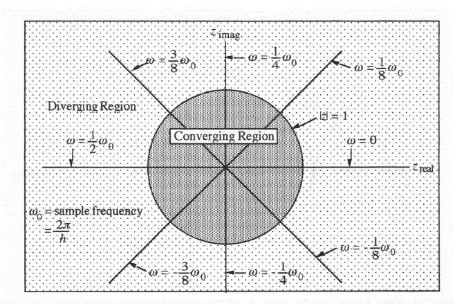
Figure 2.3. Geometric relationships between Z transform poles and the stability and frequency of the corresponding data sequences.
We now examine the stability of the digital system in Figure 2.2, which we recall represents simulation of a first-order linear system using Euler integration. For the system being simulated to be stable, it is clear that the characteristic root λ must be negative. From the digital system Z transform, H*(z), it is apparent that the single pole is given by
![]()
![]() (2.49)
(2.49)
As we vary the step size h from 0 to infinity, the pole z1 moves along the real axis from +1 to minus infinity, as shown in Figure 2.4. This plot in the z plane is analogous to the so-called root locus plot in the s plane for closed-loop systems as the controller gain constant is varied from zero to infinity. In Figure 2.4 we see that the locus crosses the unit circle in the z plane for h = -2/λ. For h > -2/λ the pole z1 lies to the left of the point z = -1, and the simulation will be unstable. The corresponding data sequence will be an exponentially growing oscillation at one-half the sample frequency. In fact, for h in the range -1/λ < h < -2/λ the pole z1, although within the unit circle, lies on the negative real axis. This means that the corresponding stable data sequence is oscillatory at one-half the sample frequency, even though the continuous system being simulated has a non-oscillatory exponential transient.
In Figure 2.5 the data points from a series of digital solutions with different integration step sizes are shown, along with the exact solution of the continuous system for x(0) = 1 and f(t) = 0. For each case the step size h corresponds to one of the values shown on the root locus plot in Figure 2.4. It should be noted that the characteristic root λ of the system considered here is related to the time constant of the first order system by the formula T = -1/λ. Thus λh = -0.2 corresponds to
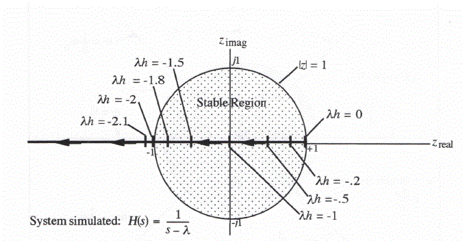
Figure 2.4. Root locus for the pole z1 of the digital system when Euler integration is used to simulate a first-order linear system with 0 < h < ∞
h = .2T, i.e., the integration step size h is equal to one-fifth the time constant T of the first-order system being simulated. Figure 2.5 shows that in this case the digital solution is quite close to the exact solution. For h = .5T the digital solution is clearly decaying more rapidly than the exact solution. This is because the characteristic root λ* of the digital system has a slightly larger magnitude than the ideal root λ, which is consistent with Eq. (2.24) for negative λ. For h = T the digital solution drops to zero at the first integration step and remains zero for all subsequent time steps. In this case the pole z1 = 0 and Eq. (2.22) shows that the equivalent characteristic root λ* (=σ) is also equal to zero. Thus the digital solution remains equal to a constant, namely zero.
For h = 1.5T and 1.8T, Figure 2.5 shows that the digital solutions are damped oscillations at one-half the sample frequency. In each case the corresponding pole z1 in Figure 2.4 lies on the negative real axis but inside the unit circle in the z plane. For h = 2T (i.e.,λh = -2) the pole in Figure 2.4 lies at z1 = -1. This results in a digital solution which is an undamped oscillation at one-half the sample frequency, which again is confirmed in Figure 2.5. Finally, for h = 2.1T Figure 2.5 shows that the digital solution is a growing oscillation, once more at one-half the sample frequency. The corresponding pole z1 in Figure 2.4 lies on the negative real axis, but outside the unit circle in the zplane. This accounts for the observed instability in the digital solution.
In considering Euler integration for simulating the second-order linear system described by Eq. (2.43), we obtained Eq. (2.46) for the digital system Z transform. Since the denominator of H*(z) is in this case a quadratic in , it is clear that H*(z) has two poles, z1and z2. These poles are related to the two characteristic roots, λ1 and λ2, of the continuous system by Eq. (2.49) for the case of both real and complex λ. We recall that λ1 and λ2 will be a complex conjugate pair when the second-order system is underdamped. For the digital simulation of the second-order system to be stable, both the Z transform poles must lie within the unit circle in the z plane. From Eq. (2.49) the stability criterion becomes
![]()
![]() (2.50)
(2.50)
Here |1 + λh| – 1 represents a unit circle centered at the origin in the 1 + λh plane or, alternatively, a unit circle centered at -1 in the λh plane. This circle is shown in Figure 4.6. It is the region within
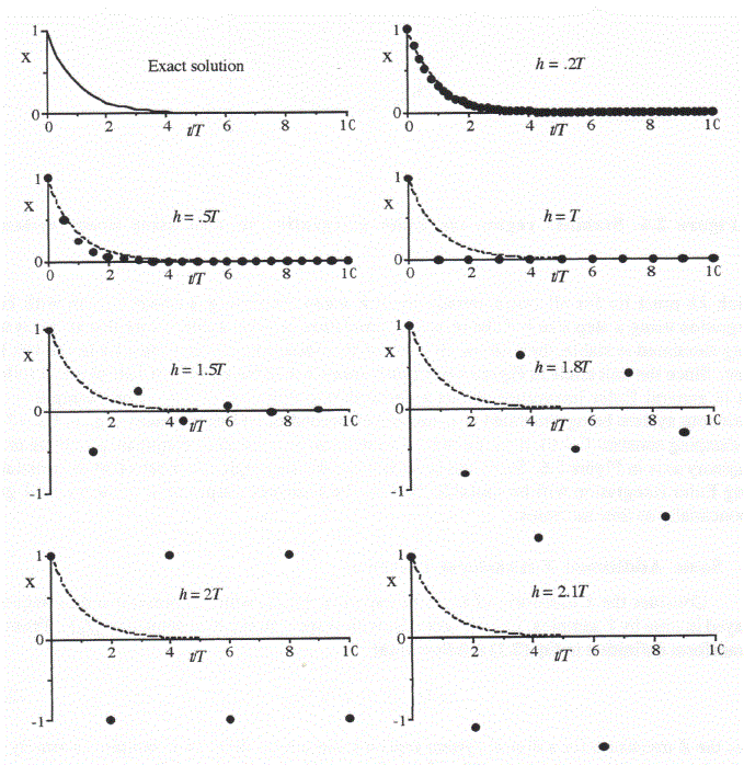
Figure 2.5. Digital solutions using Euler integration for simulating the linear system given by = λx + f(t), or, T+ x + f(t) = 0 with f(t) = 0, x(0) = 1.
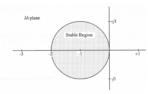
Figure 2.6. Stability region for Euler integration in simulating linear systems.
which λh must lie for all characteristic roots λ when simulating a linear system with Euler integration using a step size h if the resulting simulation is to be stable. Note that if the system being simulated is stable, then λh for all roots of the continuous system must lie in the left-half plane. Since the unit circle in Figure 4.6 is much smaller than the entire left-half plane, it follows that in general Euler integration exerts a destabilizing dynamic effect. For example, if the continuous system being simulated is an undamped second-order linear system (e.g., in Eq. (2.42) the damping constant C = 0), then the two λh values will be a complex conjugate pair lying on the imaginary axis in Figure 2.6. Since this is outside the stability region, it means that the simulation using Euler integration will be unstable, that is, the transient output data sequence will grow exponentially as time increases.
2.5 Some Additional Z-transform Formulas
Consider the Z transform of the data sequence {fn–k}, which represents a data sequence delayed in time by ksamples, i.e., kh seconds, with respect to the data sequence {fn}. From the Z-transform definition in Eq. (2.1) it follows that
![]()
![]() (2.51)
(2.51)
Thus the Z transform for a digital system representing a time delay of k samples is simply z–k. Again, it is interesting to compare these formulas with their counterparts for continuous systems. The Laplace transform of f(t – td) is given by
![]()
![]() (2.52)
(2.52)
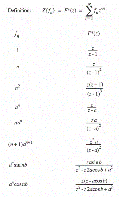
where F(s) is the Laplace transform of f(t). It follows that the Laplace transform of a continuous system representing a pure time delay, td, is e–std. Table 2.1 presents the Z transforms for a number of commonly encountered data sequences, including those already developed in this chapter.
Table 2.1
Z Transforms for Commonly Encountered Data Sequences
