Chapter 11 – Real-time Integration of State-variable Derivatives with Discontinuities

11.1 Introduction

There are many examples of dynamic systems with state-variable derivatives that have discontinuities. A simple example is a spacecraft attitude control system with on-off reaction-control thrusters. Other examples include dynamic systems with effort-limited controllers, controllers with dead-zone, etc. Also, time-dependent input functions for a dynamic system can exhibit discontinuities. This is true, for example, in the case of the digital flight control system considered in Chapter 10, where the control-surface actuator of Figure 10.8 receives a sequence of step inputs from the zero-order extrapolator. In all of these examples, the resulting discontinuities in state variable derivatives can cause very large errors when conventional numerical integration algorithms are utilized. This is because the accuracy of the numerical integration formulas is destroyed when higher-order derivatives of the state-variables do not exist. In non-real-time simulation, a variable step to the exact time of occurrence of the discontinuity can be used to retain high accuracy, providing the integration algorithm is selected carefully. In real-time simulation using a fixed time-step for integration this is not possible, and the discontinuities will in general occur at times which are asynchronous with respect to the integration frame times. In this chapter we introduce methods for handing discontinuities that preserve accurate integration when the discontinuity in state-variable derivative occurs anywhere within a given integration step.

 

11.2 Accurate Real-time Simulation in the Presence of Asynchronous Step Inputs

We first consider the case of a dynamic system with an explicit time-dependent input that exhibits step changes that can occur asynchronously with respect to a fixed integration frame rate. We have already noted above that a zero-order extrapolator, as used to convert the output of a digital controller to the input for a continuous system, will produce such step-input changes. To be sure, if we choose the integration frame rate for the continuous-system simulation to be an integer multiple of the frame rate of the digital controller, then the step discontinuities will always occur at integer step times for the continuous-system simulation. If we then integrate the step input using the Euler method, the integration will be exact. This was the scheme used in Eq. (10.2) for the actuator example in Section 10.5, where the remaining terms on the right side of the state equation were integrated using the AB-2 method. Note that the use of the AB-2 formula to integrate the step-input term will produce a very large error, one that is proportional to the first power of the integration step size h. On the other hand, the frame-rate of the digital controller may not always be fixed, in which case the step changes in input to the continuous system will indeed occur asynchronously with respect to the integer frame times of the continuous system simulation. In this case, direct Euler integration of the input will result in large errors.

 

The problem can be solved by computing the average of the input over each continuous-system integration frame. This average is then multiplied by the step size h to complete the input integration. In our actuator example of Section 10.5, this average was calculated using Eq. (10.7). In the case of an external real-time input, multi-rate input sampling can be employed, with the average input calculated using the inputs that occur within each frame of the continuous-system simulation. As the multi-rate sampling ratio N becomes large, the average calculated by a finite summation rapidly approaches the exact input average over each frame. The integration errors resulting from a finite N have already been presented in the last section of Chapter 5.

 

To illustrate the effectiveness of input averaging in handling asynchronous step inputs to a real-time simulation, we consider a second-order linear system with undamped natural frequency   and damping ratio  .  The state equations are given by

(11.1)   

 

We let the input U(t) be a unit-step that occurs at  , with  , as shown in Figure 11.1. The formula for  , the mean value of the input over the first frame, is given by

(11.2)   

 

where h is the integration step size. We now use the AB-2 method to integrate all terms except  , which is integrated by applying Euler integration to the input average  .  This results in the following difference equations:

(11.3)   

(11.4)   

 

where

(11.5)   

 

For the unit step input of Figure 11.1, we note that   for all integer frame numbers  . For  ,    and is given by Eq. (11.2). When   is an exact representation of the average value of the input U over the nth frame, the term   in Eq. (11.4) is, by definition, an exact representation of the integral.

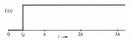
Figure 11.1. Unit step input applied at time .

 

As a specific example, we let   and  . . Eqs. (11.3), (11.4) and (11.5) are used with an integration step size h = 0.1. Figure 11.2 shows the error in simulated response for four different times of unit-step application, namely,    ,   and  .  It is clear that the error is almost unaffected by the time   at which the step input occurs. For comparison purposes, Figure 11.3 shows the errors when the AB-2 method is used for all integrations, including the input term.

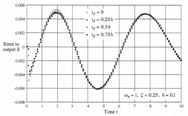
Figure 11.2. Error in simulated 2nd-order system response to a unit step input applied at different times t_d. AB-2 integration used except for the step input, which uses Euler integration of the average input over each frame.

 

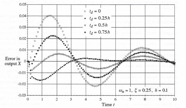
Figure 11.3. Error in simulated 2nd-order system response to a unit step input applied at different times t_d. AB-2 integration used for all terms.

 

Not only are the errors much larger (by almost an order of magnitude), but also the errors are strongly dependent on the time t_d at which the step input is applied. In fact the minimum error occurs for  ,  which means that the unit-step input is applied half-way through the first integration step. This is consistent with the observation we made back in Chapter 6, where Figure 6.12 shows that the linear extrapolation inherent in the AB-2 approximation to the state-variable derivative produces a response representative of a step which occurs one-half frame early. Thus for  , Figure 11.1 shows that the input data points are given by  . This then means that the effective step input when using AB-2 integration occurs at  , i.e., a half-step ahead of the first input sample. But this is exactly when the true continuous step input occurs when  , which explains why the error in AB-2 simulation of the second-order system is minimized. For  , which means that the unit-step input is applied one-quarter of the way through the first integration step, the input data points are again given by   and the effective step input when using AB-2 integration once more occurs at  , which is now a quarter frame behind the actual step-input time. Thus the AB-2 solution lags behind the true solution by 0.25h, which causes a negative peak error of -0.16 at t = 0.8, as shown in Figure 11.3. On the other hand, when   and the effective step input when using AB-2 integration occurs at  , which is one-half frame ahead of the actual step-input at t = 0. Thus the AB-2 simulation leads the true solution by one-half frame, which causes a positive peak error of 0.04 at t = 1.5, again as shown in Figure 11.3. Finally, for   and the effective step input when using AB-2 integration occurs at t = 0.5h, which is one-quarter frame ahead of the actual step-input time. This causes a peak error of 0.022 at t = 1.7. Thus all of the AB-2 simulation errors in Figure 11.3 can be explained qualitatively by comparing the effective step-input times with the actual step-input times, and the errors are in general quite large. Of course, the problem is all but eliminated when we utilize Euler integration of the average step input over each frame, as the results in Figure 11.2 demonstrate.

 

When the step that occurs at time   represents a real-time input, it should be noted that the occurrence of the step input cannot be observed in real time prior to  . Thus the information needed to implement the input-averaging scheme is in general not available at the beginning of each integration frame. The worst case is when   occurs just before an integer frame time, since under these conditions there is almost no time left to solve the difference equations and produce the simulation outputs in real time at the next integer frame time. However, for the second-order example here, reference to Eq. (113) shows that the output data point   for the nth integration frame depends only on the data points   and   from previous frames and not on the input for the nth frame. Thus we can provide real-time output displacement data points   for the nth frame even when the input-average information is not available until the end of the frame. However, this is clearly not the case for the output velocity data points  , which Eq. (11.4) shows do depend on the input average   over the nth frame. Put another way, if we use multi-rate sampling of the real-time input to compute  , we must wait for the last sample to occur in the nth frame, i.e., almost to the end of the frame, before the calculation can be completed. Then real-time outputs of state variables whose derivatives depend directly on the real-time input can only be furnished using the extrapolation methods described in Chapter 4 and used in Chapters 8, 9 and 10. However, the extrapolation interval can be reduced to considerably less than one frame by scheduling in the n – 1 frame all those calculations associated with the nth frame that do not depend on the real-time input for the nth frame. Indeed, this is exactly the way in which we are able, as noted above, to provide   in real time without resorting to extrapolation, even when using the input-averaging method of integration for our example simulation here.

 

It is useful to see whether the accuracy improvement for step inputs realized by replacing AB-2 with Euler integration of the average input carries over when we use AB-3 integration for the simulation. In this case the difference equations become

(11.6)   

(11.7)   

 

Here the derivative term   is again given by Eq. (11.5). In this case the results for our example second-order system are shown in Figure 11.4, where the output error is plotted versus time for unit-step inputs again occurring at  , 0.25h, 0.5h and 0.75h, in this case using Eqs. (11.5), (11.6) and (11.7) for the simulation. Comparison with the earlier AB-2 results in Figure 11.2 shows that the AB-3 errors are generally much smaller, with the exception of the startup error for the first two frames. Here the startup error is caused by the fact that the output data point   is equal to zero for the first integration frame, whereas the exact solution for a unit step that occurs at   is equal to   for  . This results in an approximate error of   for the first integration step. Since   for the AB-2 simulation as well, the first-frame errors for t = h = 0.1

 

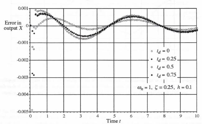
Figure 11.4. Error in simulated 2nd-order system response to a unit step input applied at different times t_d. AB-3 integration used except for the step input, which uses Euler integration of the average input over each frame.

 

in Figure 11.2 are the same as those in Figure 11.4 for AB-3. This startup error can be greatly reduced if we use third-order implicit integration to compute  . From Eq. (1.15) the formula is given by

(11.8)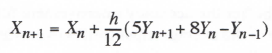   

 

Here Eq. (11.8) can be implemented after Eq. (11.7), so that   is actually available explicitly in the calculation of  . This results in the simulation errors shown in Figure 11.5, which are considerable smaller because of the reduction in startup error. Note, however, that the use of   in Eq. (11.8) makes the calculation of   dependent on the input average   over the nth frame, which in turn means that   will in general not be available in real time when U represents a real-time input.

 

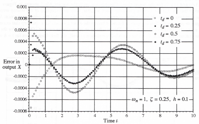
Figure 11.5. Error in simulated 2nd-order system response to a unit step input applied at  Euler method used to integrate the average input over each frame, 3rd-order implicit integration used to compute , AB-3 used for remaining integrations.

 

Figure 11.6 shows the simulation output errors when the AB-3 method is used for all integrations, including the input term. Comparison with Figures 11.4 and 11.5 demonstrates that the errors are very much larger and in fact quite comparable to those in Figure 11.3 for the AB-2 method. As in the AB-2 case, Figure 11.6 also shows that the AB-3 errors are smallest when the step input is applied half-way through the integration frame  . This is again consistent with our earlier observation in Chapter 6, where Figure 6.16 shows that the quadratic extrapolation inherent in the AB-3 approximation to the state-variable derivative produces a response representative of a step which occurs one-half frame early. Only by employing the Euler method for integrating the average input over each frame are we able to realize any improvement over the AB-2 method by using AB-3 integration.

 

Figure 11.6. Error in simulated 2nd-order system response to a unit step input applied at different times t_d. AB-3 integration used for all terms.

 

11.3 The Use of Function Averaging for Discontinuous Nonlinear Derivatives

In this section we consider discontinuous state-variable derivatives, where the discontinuity occurs as a nonlinear function of the state variables. Unless a variable step to the exact time of occurrence of the discontinuity is utilized, discontinuities in displacement or slope can cause very large errors when using conventional integration algorithms. As in the case of discontinuous explicit inputs treated in the previous section, we combine a representation of the average of the nonlinear function over each integration frame with Euler integration to provide a fast and accurate simulation. Assume that the state equation is given by

(11.9)   

 

where f(x) is a nonlinear function which can include discontinuities. For an integration step size h, the following equation represents an exact numerical integration formula:

 

(11.10)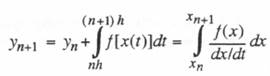 

 

We next assume over the interval of integration that the time derivative of x, dx/dt, is a constant which can be represented by the following central-difference approximation:

(11.11) 

 

Then Eq. (11.10) can be rewritten as

 

(11.12) 

 

where

(11.13)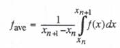 

 

With Eq. (11.13) we have converted the integral of  f(x) with respect to t in Eq. (11.10) to an integral with respect to x. In fact   is simply a representation of the average value of f(x) over the interval of integration, which corresponds to one integration frame. For any specified f(x) the integral is a function of   and  . For example, if f(x) = x, a linear function, the   function becomes

(11.14)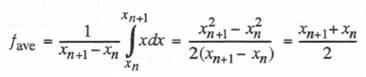 

 

In this case we see that Eq. (11.12) represents trapezoidal integration. However, when f(x) is a nonlinear function of x, Eqs. (11.12) and (11.13) will produce a result that is more accurate than trapezoidal integration produces when applied to f(x)

 

It should be noted that  , as defined in Eq. (11.13), is undefined for  . In this case it is clear that   should be equal to  , the value of f(x) for  . In an actual simulation this can be implemented by a conditional statement that sets   equal to   when  ; otherwise,   is given by Eq. (11.13).

 

Figure 11.7 illustrates some typical discontinuous nonlinear controller functions. For each of these functions we now proceed to derive analytic formulas for  , as defined in Eq. (11.13). Consider first the bang-bang control or switch function shown in Figure 11.7a. The function can be represented analytically by the formula  . From Eq. (11.3) it follows that

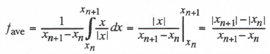
(11.15)

 

 

Note that if both   and   are positive,  , whereas when both   and   are negative,  . When   and   have opposite polarity,   will be somewhere between +1 and -1, and will represent the average value of the switch function over the interval  ,  .

 

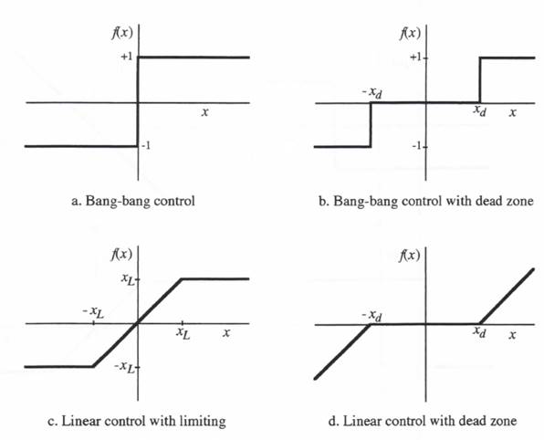
Figure 11.7. Typical controller discontinuous nonlinearities.

 

Next consider the linear function with limiting, as shown in Figure 11.7c. Here the function can be represented analytically by the formula  . From Eq. (11.13) we obtain the following formula for  :

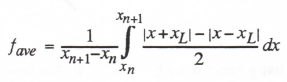
or

(11.16)

 

Consider next the derivation of the   function for the bang-bang control with dead zone, as illustrated in Figure 11.7b. Figure 11.8a shows how this function can be represented as the superposition of two bang-bang switch functions with inputs biased by   and  , respectively. It follows from Eq. (11.15) for the individual   functions that the overall   function representing bang-bang control with dead zone is given by

 

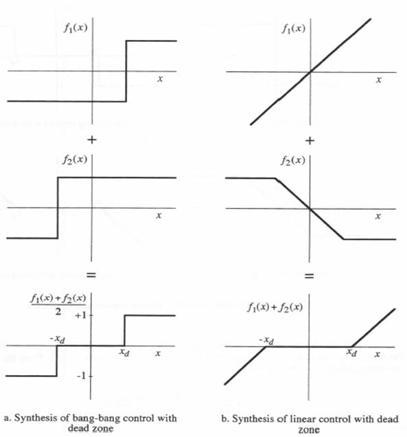
Figure 11.8. Synthesis of discontinuous control functions.

 

(11.17)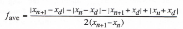 

 

Similarly, the linear function with deadzone illustrated in Figure 11.8b can be represented as the superposition of a pure linear function and an effort-limited linear function, as shown in Figure 11.8b. Thus we can write the following formula for the   function:

(11.18)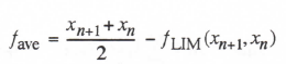             

 

Here   represents the   function given in Eq. (11.16) for the linear control with limiting, and   is the   function given in Eq. (11.14) for the pure linear function.

 

11.4 General Synthesis of Analytic Averaging Functions

From the example in Figure 11.8a it is evident that any symmetric nonlinear function can be synthesized by a superposition of bang-bang switch functions, each with an appropriate weighting constant and input bias. Also, from the example in Figure 11.8b it is apparent that any symmetric nonlinear function with slope discontinuities can be synthesized by a superposition of linear functions with limiting, each with an appropriate weighting constant and input-limit bias. Symmetric nonlinear functions consisting of both straight-line segments and displacement jumps can be synthesized by a superposition of both linear functions with limiting and bang-bang switch functions. In all cases the corresponding   function can be written in terms of the   functions given in Eqs. (11.15) and (11.16).

 

We next consider asymmetric nonlinear functions with displacement discontinuities. These can in general be synthesized by a superposition of step functions. The individual unit step function d(x) in Figure 11.9a can be represented analytically by the formula  . From Eq. (11.13) the corresponding   function is given by

(11.19)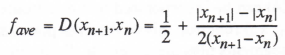 

 

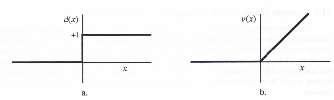
Figure 11.9. Unit step and ramp functions.

 

Any staircase-type discontinuous function can be represented as the weighted sum of unit-step functions with biased inputs. Thus we can write

(11.20)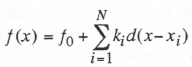 

 

The corresponding   function can be written in terms of the   function given in Eq. (11.19). Thus

(11.21)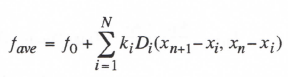 

 

Following the same procedure, we can synthesize any asymmetric nonlinear function consisting of straight-line segments by a sum of unit-ramp functions with biased inputs. The unit-ramp function   in Figure 11.9b can be represented by the formula  . From Eq. (11.13) the corresponding    function   is given by

(11.22)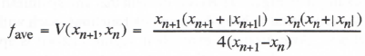 

 

The nonlinear function consisting of straight-line segments can be represented by the formula

(11.23)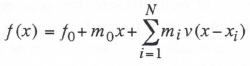 

 

It follows that the corresponding formula for the   function is given by

(11.24)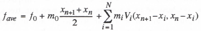 

 

Eqs. (11.19) through (11.24) can be incorporated into a computer subroutine which will automatically calculate the   function, given the data points that define any nonlinear function   that consists of linear segments plus displacement discontinuities.

 

11.5 Example Simulation of a Bang-bang Control System

To illustrate the superiority of the   scheme over conventional integration methods in the simulation of dynamic systems with discontinuous nonlinearities, we now consider the bang-bang control system illustrated in Figure 11.10. The feedback system consists of a pure-inertia plant driven by a bang-bang controller with hysteresis, with proportional plus rate control provided by the lead/double-lag filter shown in the figure. If the controller were also to include dead zone, the system would be representative of a typical spacecraft single-axis reaction jet attitude control system.

 

For the parameters shown in the figure, the transient response of the control system for zero input (r = 0) is shown in Figure 11.11 for two different initial conditions c(0) in output displacement. The other three states are initially zero. Note that the response approaches a limit cycle in both cases. This is of course typical for any bang-bang control system.

 

The proportional-plus-rate filter used in our example here is identical to the controller we first introduced in Eq. (6.25) to illustrate the special techniques considered in Chapter 6 for simulating linear systems. The usual method for writing the state equations that represent the filter is based on equations for simulating the second-order transfer function without the rate term  . In this case the state equations become

 

(11.25) 

 

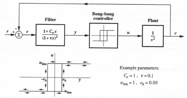
Figure 11.10. Bang-bang control system with hysterisis.

 

 

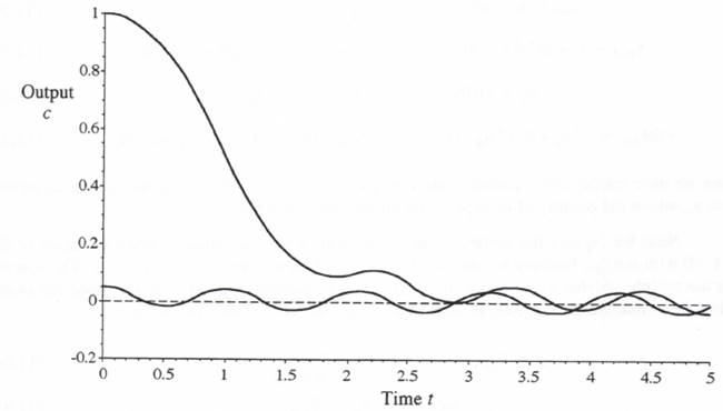
Figure 11.11. Transient response of bang-bang control system for two different initial conditions.

 

The filter output y is then given by

(11.26) 

 

For our example simulation here we will chose the state variables such that one of the variables represents the filter output directly. Thus we let

(11.27) 

 

If we differentiate   in Eq. (11.27), the resulting second-order differential equation is a direct representation of the proportional-plus-rate filter. The remaining state equations can be written as

(11.28) 

 

The SIGN function utilized here is defined as follows:

(11.29) 

 

The definition of SIGN(X) for X =0 is unimportant in our bang-bang example, since there is zero probability that X will be exactly zero in either a real system or actual simulation.

 

We first consider the simulation of the system using the AB-2 method for all integrations. The difference equations are the following:

(11.30) 

(11.31) 

(11.32) 

(11.33) 

 

Here we have introduced a discrete state variable   in order to mechanize the hysteresis bias  , where the polarity of   depends on the previous switch state  .

 

Next we replace the conventional evaluation of the bang-bang control function in Eq. (1132) with the   function by utilizing Eq. (11.15), followed by Euler integration. The formula for the switch variable   given in Eq. (11.32) is still retained to preserve the method for evaluating the switch bias,  . But the equations for   and   are replaced by

(11.34)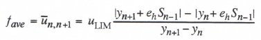 

(11.35) 

In Eq. (11.34) we have denoted the   function by   to indicate that it represents the average value of the controller output u over the nth frame. This average value is then multiplied by the step size h in Eq. (11.35) to produce the incremental change in cdot over the nth frame. Thus Eq. (11.35) is a form of modified Euler integration.

 

In Figure 11.12 the error in simulated control system output c with c(0) = 1 and step-size h = 0.05 is plotted as a function of time. Two cases are shown. In one case the standard AB-2 method is used for all integrations, which means that Eqs. (11.30) through (11.33) are employed for the simulation. In the other case the average output of the controller is combined with Euler integration, as given in Eqs. (11.34) and (11.35), to compute the plant velocity, cdot, while the AB-2 method is used for the other three integrations. The same two cases are repeated in Figure 11.13, which shows the output errors with the smaller initial condition, c(0) = 0.05. Both figures clearly demonstrate that the output-averaging scheme, when applied to our bang-bang control example, makes an enormous improvement in the accuracy of the simulation. Later in this chapter we will show how the accuracy can be further improved by using a variable integration step directly to each bang-bang controller switch time, even when the simulation must be performed in real time.

 

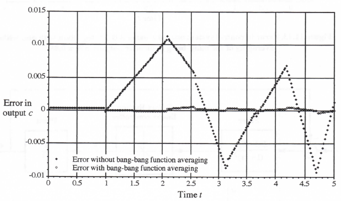
Figure 11.12. Error in control system output c using AB-2 integration with and without averaging of the bang-bang controller output; c(0) = 1.

 

11.6 Example Simulation of an Effort-limited Control System

As a second example to illustrate the superiority of the   scheme over conventional integration, we consider the linear control system with effort limiting that is illustrated in Figure 11.14. The control-system configuration is identical to our earlier example in Figure 11.10, with the exception that we have substituted a linear controller with effort limiting for the bang-bang controller. Also, we have added a gain constant K to the filter which provides proportional-plus-rate

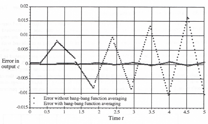
Figure 11.13. Error in control system output c using AB-2 integration with and without averaging of the bang-bang controller output; c(0) = 0.05.

 

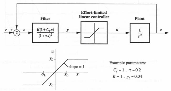
Figure 11.14. Linear control system with effort limiting.

 

control. It should be noted that any physical control system will have some type of effort limiting associated with the controller, so that a nonlinearity similar to that considered here will invariably be present in a realistic simulation. As noted earlier, the slope discontinuities in the controller function can cause large errors when using conventional integration methods, as we shall demonstrate with our example here.

 

For the parameters in Figure 11.14, the transient response of the control system with zero input (r = 0) and zero initial conditions for all states except the controller output, where c(0) = 1, is shown in Figure 11.15. Also shown is the case where there is no effort limiting. Note that the effort limiting given by   makes a very large difference in the initial transient compared with the transient when no effort limiting is present and the control system is completely linear. Only for t > 45 in Figure 11.15 has the solution for the effort-limiting case damped to the point where the transient becomes linear.

 

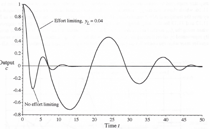
Figure 11.15. Transient response of control system with and without effort-limited control.

 

We use the following state equations to represent the system:

(11.36)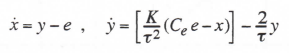 

(11.37)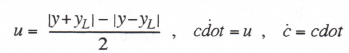 

 

As in the previous example, we first consider a simulation of the effort-limited control system using the AB-2 method for all integrations. In this case the difference equations are the same as those given earlier in Eqs. (11.30) through 11.33), except that the formula for u in Eq. (11.37) is used to calculate   from  . We next replace the conventional evaluation of the effort-limited linear control function with the   function given by Eq. (11.16), followed by Euler integration. In the notation for our example here, the formula for   becomes

(11.38)

 

As in the previous example, Eq. (11.35) is used to calculate  .

 

We now examine the output errors when the effort-limited controller is simulated (1) entirely with AB-2 integration, and (2) with AB-2 integration except for the use of controller-output averaging plus Euler integration for the calculation of cdot. The simulation parameters are the same as those used for the effort-limited reference solution in Figure 11.15, including a controller limit given by  . We use a step size h = 0.1 for both simulations instead of the much smaller step size employed to obtain the reference solution. The results are plotted versus time in Figure 11.16, which shows that the   method provides a substantial improvement in simulation accuracy over the traditional AB-2 simulation. However, comparison with the earlier results in Figures 11.12 and 11.13 for the bang-bang control system shows that in Figure 11.16 the improvement when using the   method is less dramatic. This is undoubtedly due to the less severe nonlinear-ity represented by effort limiting in comparison with bang-bang control, which in turn results in a smaller error when the controller output is integrated using a standard algorithm such as AB-2.

 

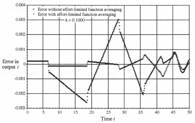
Figure 11.16. Error in control system output c using AB-2 integration with and without averaging of the effort-limited controller output; h = 0.1.

 

Since the errors resulting from controller discontinuities will be dependent on where each discontinuity occurs with respect to the integer frame times, it is useful to examine the simulation errors when the step size h is changed very slightly from the nominal value of 0.1 used for the simulations in Figure 11.16. This will have the effect of shifting the time of discontinuity within the individual integration steps. This has been done in Figures 11.17 and 11.18, where we have plotted the simulation errors with and without the  , method for step sizes given by h = 0.1005 and 0.1010. These step-size changes from the nominal value of h = 0.1000 are large enough to make significant shifts in the discontinuity times with respect to the integer frame times, and yet are small enough that they cause negligible increases in simulation errors due the increased step size. Comparison of Figure 11.17 with Figure 11.16 shows that the error for the simulation that uses the AB-2 method for all integrations has been reduced significantly, even though the integration step size has been increased from h =0.1000 to h = 0.1005 (note the difference in vertical scales between the two figures). However, the error for the simulation that uses the  , method followed by Euler integration is almost unchanged when the step size is increased from 0.1000 to 0.1005. On the other hand, comparison of Figure 11.18 with Figure 11.16 shows that the error for the simulation that uses the AB-2 method for all integrations has increased as a result of the change in step size from 0.1000 to 0.1010. Once again, however, the error for the simulation that uses the   method followed by Euler integration is almost unchanged when the step size is increased from 0.1000 to 0.1010. This lack of error dependence on time of discontinuity with respect to integer frame times is more evident in Figure 11.19, which shows on a common plot the simulation errors when using the   method with h = 0 .1000 , 0.1005, and 0.1010. This clearly demonstrates the

 

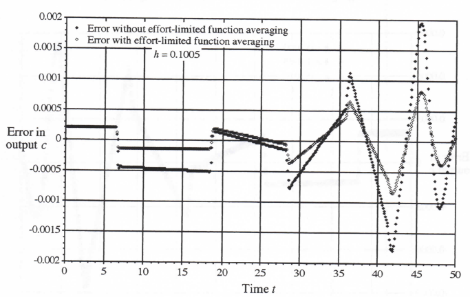
Figure 11.17. Error in control system output c using AB-2 integration with and without averaging of the effort-limited controller output; h = 0.1005.

 

Figure 11.18. Error in control system output c using AB-2 integration with and without averaging of the effort-limited controller output; h = 0.1010.

 

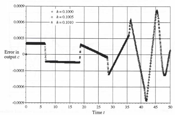
Figure 11.19. Error in control system output c using AB-2 integration along with averaging of the effort-limited controller output, Euler integration; h = 0.1000, 0.1005, 0.1010.

 

effectiveness of the   method in reducing the sensitivity of the simulation error to discontinuities in state-variable derivatives.

 

11.7  Use of a Variable Step to the Time of Discontinuity in Real-time Simulation

Thus far in this chapter we have described how the average value of a discontinuous state-variable derivative function over a fixed time step can be combined with Euler integration to maintain accuracy in real-time simulation, with the remaining integrations accomplished using predictor methods. In this section we consider an alternative technique to maintain accuracy in the real-time simulation of dynamic systems with discontinuous state-variable derivatives, namely, the use of a variable integration step directly to the time of discontinuity. Although this technique has been widely used in non-real-time simulations, it has not in general been employed in real-time simulations because of the requirement to depart from a fixed integration step size. However, in Chapter 9 we have seen that variable-step integration can in fact be utilized quite effectively in real-time simulation, providing the step size is chosen so that the simulation on average keeps up with real time. Extrapolation formulas are then used to produce a fixed-step, real-time output, with the preferred extrapolation algorithm based on the same predictor integration method used in general for the real-time integrations.

 

To explain how the variable step to the time of discontinuity works in real time, assume that the discontinuity occurs when X is equal to zero, where X is either a state variable or a function of state variables. At the start of the nth integration frame, the time increment   at which X will next be equal zero, i.e., the time increment until the next discontinuity occurs, is calculated. When X is a state variable, this calculation can be based on the integration formula used to compute  , with the step size in the integration formula given by  . When X is a function of state variables,   is calculated by using an appropriate extrapolation formula. This calculation can either be accomplished by an explicit analytic equation or, if that is not possible, by an iterative procedure. Once calculated, the time increment   is compared with  , the nominal fixed integration step size used for the real-time simulation. If  , the step size   for the nth integration step is set equal to  .  Thus an additional integration step is taken using the nominal fixed-step size. On the other hand, if   , the step size   for the nth integration step is set equal to  . It follows that the time   corresponding to the end of the nth integration step will now be equal to  , i.e., the time at which the discontinuity occurs. Thus we will have implemented a variable step to the time of discontinuity. This variable step will clearly lie in the range  .  If we assume that   is equal to the execution time for each integration frame calculation in the simulation (this will be true when we are running the real-time simulation at the maximum possible frame rate), it follows that at the end of the nth frame, the simulation results will actually be ahead of real time by the increment  .  To restore the simulation outputs to coincide with real time at the end of the following step, we set   equal to  .  The procedure for accomplishing all of this will be clarified when we consider the specific example in the next section.

 

It should be noted that an alternative algorithm for determining the step to the next discontinuity is based on setting   equal to   when   instead of  .  In this case the variable step to the discontinuity will clearly lie in the range  .  Now, however, at the end of the nth integration frame the simulation results will clearly have fallen behind real time by the increment  . The only way a real time output corresponding to   can be obtained is by extrapolation. But this will involve extrapolation over the time of discontinuity,  , which can lead to large errors. By implementing the variable step   to the discontinuity when   instead of  , we ensure that the simulation result at the end of the nth frame is ahead of real time, in which case interpolation over an interval that does not include the discontinuity can be used to obtain the real-time output corresponding to the time  .

 

11.8 Example of a Two-degree-of-freedom System with Nonlinear Friction

To illustrate the methodology described above for implementing a variable step to the time of discontinuity, we consider the problem of simulating a two-degree-of-freedom dynamic system which includes dry friction with a breakaway force that exceeds the running force. The mechanical system used as an example is shown in Figure 11.20. It can be considered to be a simplified model of an automobile suspension system, where   represents the sprung mass,   the unsprung mass, and x(t) the vertical displacement of the road. The suspension system is represented by the spring with rate-constant   and the shock absorber with viscous-damping constant  . In addition, the effect of dry friction in the suspension system is represented by the friction force   shown in the figure. The compliance and damping of the tire are represented by the constants   and  , respectively. Vertical displacement of   is denoted by   and   is the vertical displacement of  . The fixed reference points for   and   are chosen such that   when x = 0 and the two masses are in static equilibrium. In this way we can eliminate consideration of the constant gravity force acting on the masses.

 

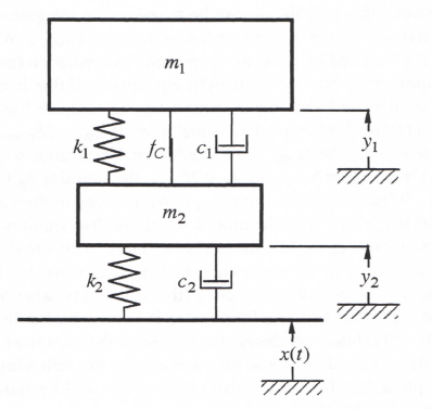
Figure 11.20. Example two-degree-of-freedom system.

 

Summing the vertical forces acting on   and   in Figure 11.20, we obtain the following equations of motion:

(11.39) 

(11.40) 

 

In writing Eqs. (11.39) and (11.40), we have assumed that the forces in Figure 11.20 are positive downward. When the relative velocity   is positive, the dry-friction force   acting on the mass   is directed downward and therefore appears as   in Eq. (11.39). On the other hand, the dry-friction force   acting on the mass   for   positive is directed upward and therefore appears as   in Eq. (11.40).

 

It is more convenient to implement Eq. (11.39) in terms of relative displacement  . If we subtract   from both sides of Eq. (11.39) and substitute y for  , we obtain

(11.41) 

 

Eqs. (11.40) and (11.41) then represent the equations that must be integrated numerically to simulate the two-dof system.

 

We now define the dry friction model which will be used in the simulation. When the relative velocity  , we will assume that the friction force  , i.e., +C when   and –C when  . Here C is the magnitude of the sliding friction force. When  , the two masses will either stick or not stick together, depending on whether the required sticking force magnitude is less or greater than the breakaway force magnitude  . Thus it is necessary to determine the sticking force   required to hold the two masses together when  . When the masses are stuck together,  . With this substitution made in Eq. (11.41) and   replaced by  , we can solve for the required sticking force,   . Thus

(11.42) 

 

We can now define the friction force   as follows:

(11.43)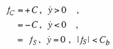 

 

When   and  , sticking will not occur and the relative velocity   an instant later will take on the polarity of  . Thus we write

(11.44) 

 

When the relative velocity   and at the same time the magnitude of the force   required to hold the two masses together exceeds the breakaway force  , Eq. (11.44) indicates that the relative velocity   an instant later will have the polarity of   and hence produce a friction force given by  . For example, assume that   and   (i.e., the required force to hold   and   together in Figure 11.20 acts downward on   and exceeds the breakaway force). It follows that the mass   will then move upward with respect to  , corresponding to a relative velocity  .

 

When sticking occurs and the two masses are held together by the friction force, the number of degrees of freedom reduces from two to one. In this case, summing the vertical forces acting on the combined, two-mass system results in the following equation of motion:

(11.45) 

 

We note that when   in Eq. (11.40) is replaced by the formula for   in Eq. (11.42), the resulting equation is identical with Eq. (11.45). Thus Eq. (11.45) is consistent with the original equation of motion for   when the friction force is replaced by the sticking force required to hold   and   together.

 

11.9. Difference Equations for Simulation

Next we consider the difference equations used in the numerical simulation of the example two-dof system, including the friction force as described above. In order to avoid double subscript notation, we introduce the following new symbols for the state variables:

 

From Eqs. (11.40), (11.41) and (11.45) the state equations can then be rewritten as

(11.46) 

 

where the state variable derivative formulas are given by the following equations:

(11.47) 

(11.48)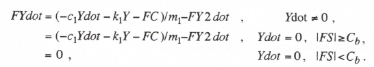 

(11.49) 

(11.50)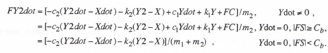 

 

Here the symbols X and Xdot have been used instead of x and  , respectively; also, FC and FS replace   and  , respectively. From Eqs. (11.42) through (11.45) the formulas for FC and FS become

(11.51) 

(11.52)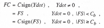 

 

 

11-24

 

Once again we note that FS in Eq. (11.51) represents the friction force required to keep mass   stuck to mass  .

 

Having rewritten the state equations with new symbols, we now convert these to the difference equations for the numerical simulation. In general, the integration step size used for the simulation will be fixed, and we will employ the AB-2 second-order predictor algorithm. However, when a friction force discontinuity is encountered, the step size will be changed as necessary to have the integration frame end at the time of discontinuity. Thus it becomes necessary for us to utilize the variable-step version of the second-order predictor method, first introduced in Chapter 10. For example, when applied to the state equation   in Eq. (11.46), the variable-step formula for computing the state   at time   from the state   at time   is the following:

(11.53)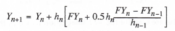 

 

Here   is the step size of the nth integration frame. For  , we note that Eq. (11.53) reduces to the fixed-step AB-2 formula. We have already noted in Chapter 10 that the coefficients of   and   in Eq. (11.53) need only be calculated once each frame, regardless of the number of state variables to be integrated, after which implementation of Eq. (11.53) for each state variable requires only two multiplications and two additions, the same as for fixed-step AB-2 integration. The remaining state equations in (11.46) take the same form as Eq. (11.53).

 

The step size   for which the relative velocity   will vanish at the end of the nth frame can be determined by setting   when Eq. (11.53) is rewritten for  . This results in the following quadratic in  :

(11.54) 

 

where

(11.55)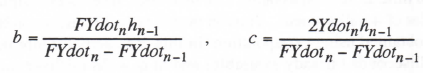 

 

The solution to Eq. (11.54) is simply

(11.56) 

 

where the + or – sign is selected such that . For most integration frames the step size   will be equal to a constant nominal step size,  . As noted earlier in Section 11.7, it is only when the time increment  , until the next occurrence of the discontinuity falls within the range   that the step size   for the nth integration frame should be set equal to the   value given by Eq. (11.56). Since a sign reversal in the relative velocity Ydot within any integration frame indicates that Ydot has passed through zero during the frame, we can examine the product   with   set equal to   to determine whether such a sign reversal will take place. In particular, if    for  , the discontinuity will not occur prior to the time  , and   should be set equal to   for the nth integration step. On the other hand, if    for  , the discontinuity will occur prior to the time  , and   should be set equal to  , as given by Eqs. (11.55) and (11.56). This will result in an integration step directly to the time of the discontinuity, with the step size   ranging between   and  . Since   now exceeds the execution time   for the nth frame, the simulation outputs at the end of the nth frame will be available ahead of the corresponding real time,  . Accurate interpolation based on the   and previous frame states can then be used to calculate the real-time output at time  , which is prior to the occurrence of the discontinuity. If we let the step size for the   frame be given by  , it follows that  , and the simulation outputs will have been restored to real time.

 

To avoid the startup problem with predictor integration following a discontinuity, Euler integration is used for the frame following the step to the discontinuity. Thus the formula for   is given by

(11.57) 

 

Similar Euler formulas are used for the   integration frame of the other state variables. Subsequent integration frames return to the AB-2 algorithm with step size  , until the next occurrence of a friction-force discontinuity.

 

A simple example can be used for illustration purposes. Assume that the execution time for each frame in a given simulation is 4 milliseconds; it follows that we let   milliseconds for the real-time simulation to run at its maximum frame rate, i.e., minimum integration step size. Until a discontinuity is encountered, both simulation outputs and real-time outputs occur simultaneously, every 4 milliseconds. Next, suppose that the relative velocity Ydot reverses sign at t = 33.6 milliseconds. Using the scheme described above, this will be detected in the nth frame which starts at t = 28 milliseconds, as indicated by the reversal in polarity of   at t =36 (28 + 2 ) compared with   at t = 28 milliseconds. The step size required to make   at the end of the nth frame is then given by   = 5.6 milliseconds, as computed from Eqs. (11.55) and (11.56). The resulting states, corresponding to a simulation time of 33.6 milliseconds, are actually obtained in real time at 32 milliseconds. The real-time, fixed-step output is, of course, required at integer multiples of 4 milliseconds. Thus an output at t =32 milliseconds must be calculated. This output can be obtained using extrapolation (in this case actually interpolation) based on states at   = 33.6 milliseconds (already available) and at   = 28 milliseconds (previously computed). Since the discontinuity does not occur until t = 33.6 milliseconds, the interpolated values at t = 32 milliseconds will be accurate. The next required real-time output occurs at t = 36 milliseconds, which coincides exactly with the simulation output at   when we let the step size for the Euler startup frame be given by   milliseconds. Step sizes for subsequent AB-2 integration frames continue to be set equal to   (4 milliseconds) until the next discontinuity is encountered.

 

When we have integrated Ydot to zero at the end of the nth frame, as described above, and sticking occurs because  , the two masses will continue to stick together for additional integration steps until  . During this time the relative velocity Ydot remains zero, the relative displacement Y remains fixed, and the third equation in (11.50) defines the acceleration of the single-dof system consisting of   and   stuck together. When unsticking does take place, discontinuities in state variable derivatives will once more occur. Thus it again becomes important to integrate to the exact time, or at least a close approximation to the exact time, at which unsticking occurs. This will correspond to the time at which the sticking force FS increases in magnitude to the breakaway force  .

 

Earlier in Eqs. (11.55) and (11.56) we were able to derive analytic formulas for calculating the step size   such that the relative velocity Ydot goes exactly to zero at the end of the nth frame. For the unsticking case considered here, it is not possible to derive a simple analytic formula for the required step size   to make  . Instead, we must rely on extrapolation. If, during the nth frame, the required sticking force FS is increasing, as indicated by a positive polarity for  , it follows that unsticking will occur when  . Conversely, when  , the sticking force FS will be decreasing during the nth frame, and unsticking occurs when  . Thus the force FS required for unsticking to occur is given by  . When we use quadratic extrapolation to estimate   and set the result equal to  , the equation can be written as the following power series:

(11.58) 

 

In terms of  ,   and   the following central difference approximations for   and   are obtained:

(11.59)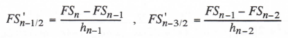 

 

The formulas for approximations to the time derivatives  and   then become

(11.60)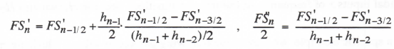 

 

From Eq. (11.58) we can solve for   using a formula similar to that given in Eq. (11.56). As a result we obtain the step size   for unsticking to occur at the end of the nth frame. Clearly, Eqs. (11.58), (11.59) and (11.60) need only be implemented for those frames within which the two masses   and   are stuck together, as indicated by   and  . If the   computed in this way is greater than  , then   should remain equal to  , the nominal step size used in fixed-step integration, and unsticking will not occur in the nth frame. However, when the   computed from Eq. (11.58) falls below   in magnitude, we utilize this   rather than   as the step size in the numerical integration formulas for the nth frame. As in the case of the previous discontinuity, this step size   will fall between   and  , and will result in the calculation of states at the instant unsticking occurs (at least to within the accuracy of the quadratic extrapolation formula). Since this event results in discontinuous state-variable derivatives, we again shift from the second-order predictor integration algorithm to an Euler-integration startup for the n+1 frame. If, as before, we let   for this Euler step, the simulation will be back on real time at the end of the n+1 frame. Subsequent integration frames employ AB-2 integration with step size   until another discontinuity is encountered. As in the case of the previous discontinuity, the real-time outputs at   are obtained using extrapolation based on states at the n + 1 and prior frames.

 

11.10. Frequency Response

In this section we consider the response of the two dof system to a sinusoidal input of road displacement, x(t). The resulting transfer functions for the sprung mass   and the unsprung mass   will give us insight into the system behavior, and also will be helpful in the later selection of a test input to illustrate the use of the numerical techniques introduced here to handle the nonlinear friction force between the two masses. In determining the sinusoidal transfer functions, we will neglect the nonlinear friction force   . It is also convenient to define the following frequency and damping parameters:

(11.61)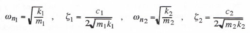 

 

In terms of these parameters it is straightforward to derive from Eqs. (8.1) and (8.2) the following formulas for the transfer operators relating the upper and lower mass displacements   and   respectively, to the road-displacement input x(t):

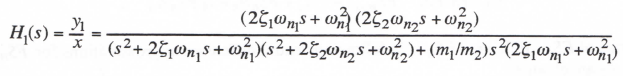
(11.62)

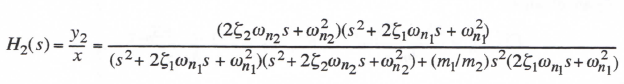
(11.63)

 

For sinusoidal inputs x of frequency  , the transfer functions become   and  , respectively.

 

As a specific example, we choose the following parameter values, which are representative of one-half the front end of a typical passenger car:

 

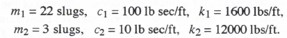
These result in the following values for the frequencies and damping ratios defined in Eq. (11.61):

 

For these parameter values Figure 11.21 shows plots of the transfer function gains,   and  , versus  . Note how the gain of the upper, unsprung mass displacement   falls off beyond about 10 rad/sec. This demonstrates the function of the suspension system, namely, to isolate the sprung mass from high-frequency road-displacement inputs.

 

When the effect of the friction force   is taken into account for sinusoidal inputs, there will be a fraction of each response cycle over which the two masses are stick together. This will have the effect of reducing the isolation of the upper mass from the high-frequency road-displacement inputs. For any given frequency, the smaller the amplitude of sinusoidal input, the larger the cycle fraction over which the two masses remain stuck together. Thus inclusion of the friction force   will make the transfer function gains dependent on the amplitude as well as the frequency of the input road displacement.

 

Based on the above considerations and the frequency response curves in Figure 11.21, we will utilize the following road-displacement function x(t) as a test simulation input:

(11.64) 

 

Reference to the plot in Figure11.22 for   shows that x(t) in Eq. (11.64) provides a sinusoidal test input with a smooth startup, i.e., no jump in initial displacement or velocity. For given values of friction force parameters, C and  , the amplitude A of the test input can be varied to demonstrate different amounts of sticking between the two masses.

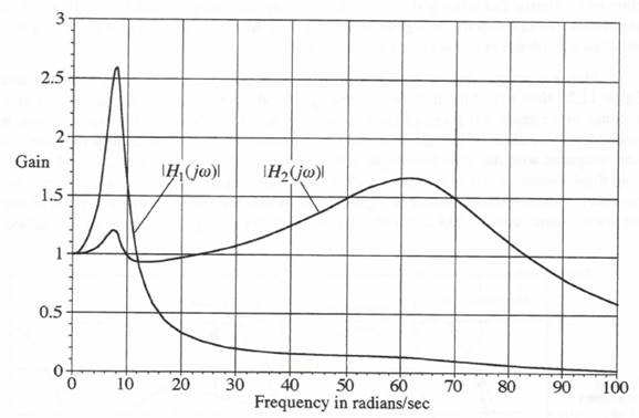
Figure 11.21. Frequency response of sprung and unsprung masses, as given by  and , respectively.

 

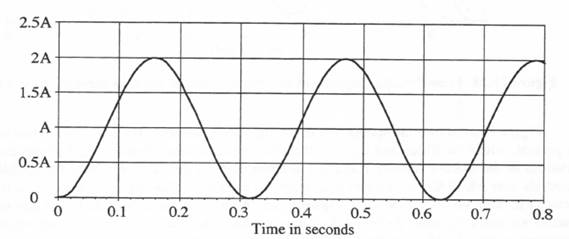
Figure 11.22. Simulation test input displacement,  .

 

11.11 Example Simulation

We now turn to an example simulation of the two dof system. In addition to the parameters given above in Section 11.10, we let the running friction force C = 20 lbs and the breakaway friction force   = 25 lbs. To obtain reference solutions, we choose a nominal integration step size   = 0.000125 seconds and use the difference equations presented above in Section 11.9, including the variable-step AB-2 predictor algorithm for direct integration to discontinuity times followed by startup Euler integration for the next integration step. With   = 0.000125 seconds the solution errors are quite negligible compared with the errors that occur when using the larger step sizes considered in our subsequent real-time simulations.

 

First we present the results when no friction is present, i.e.,  . For this case, Figure 11.23 shows the time histories for the upper and lower mass displacements, Y 1 and Y 2, in response to the input x(t) given in Eq. (11.64), which is also shown in the figure. Note that the oscillatory component of the sprung mass displacement Y l (t) is significantly reduced in amplitude compared with the 20 rad/sec input x(t), whereas the oscillatory component of the unsprung mass displacement Y 2 (t) is almost equal to the input amplitude. This is consistent with the frequency response shown earlier in Figure 11.21, where the transfer function gains of the upper and lower masses equal 0.333 and 0.971, respectively, for an input frequency of 20 rad/sec.

 

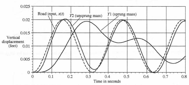
Figure 11.23. Time-domain response of two dof system; no friction force .

 

Figure 11.24 shows the sprung and unsprung displacements, Y l (t) and Y 2 (t), when friction is present, with C = 20 lbs and   = 25 lbs. For the same case, Figure 11.25 shows the time histories of the relative velocity   and displacement Y of the two masses. Note the sizable time intervals over which the two masses stick together, as exhibited by the segments of zero relative velocity in the   versus t response of Figure 11.25. As pointed out in Section 11.8, when the two masses are stuck together, the two-dof system is reduced to a single-degree-of-freedom system governed by Eq. (11.45). For the list of parameters following Eq. (11.63) and used in the example here, the undamped natural frequency of the resulting one-dof system is equal to 21.9 rad/sec

 

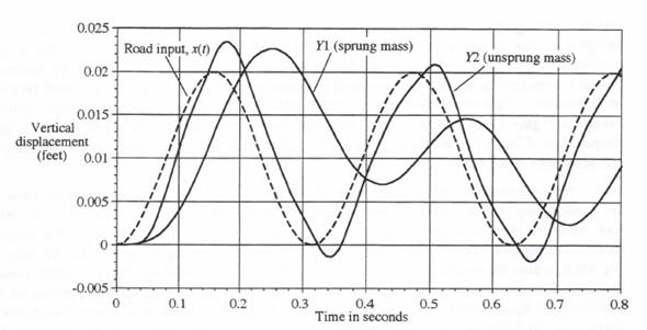
Figure 11.24. Time-domain response of two dof system; running friction force C = 20 lbs, breakaway force  = 25 lbs.

 

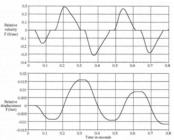
Figure 11.25.  Time history of relative velocity and displacement; running friction force C = 20 lbs, breakaway force  = 25 lbs

 

and the damping ratio is 0.0091. This very low damping ratio results from the fact that the only damping acting on the two masses, when stuck together, is that provided by the tire damping coefficient,  . Thus for the fraction of each oscillatory cycle over which sticking occurs, the system is very lightly damped with a natural frequency approximately equal to the input frequency of 20 rad/sec. This accounts for the significantly increased amplitude of oscillatory transient evident in Figure 11.24 when compared with the results for no friction in Figure 11.23. Clearly, the presence of friction in the suspension system has a deleterious effect on the high-frequency ride characteristics of the car.

 

Next we consider the simulation results for significantly larger integration step sizes than the nominal step size of 0.000125 used to generate the reference solutions shown thus far. As before, we utilize the difference equations of Section 9, including the variable-step AB-2 algorithm for direct integration to discontinuity times followed by startup Euler integration for the next step. We will examine the results for two different step sizes,   = 0.004 and   = 0.002 seconds. From the respective solutions for these integration step sizes we can subtract the reference solution obtained with   = 0.000125 in order to calculate and plot the simulation errors at each discrete frame time. In doing this, we must remember that the simulation method used here departs from fixed integration steps every time a friction discontinuity is encountered. This is necessary in order to step directly to the time at which the discontinuity occurs, after which the step size is again changed to restore the discrete simulation times to integer multiples of  .

 

Table 11.1 helps in understanding the sequence of step sizes used to implement the simulation. Shown in the table is a listing of the frame times   and associated step sizes   for the two simulation cases to be considered here, with   = 0.004 and   = 0.002, respectively. Consider, for example, the simulation with   = 0.004. Reference to Figure 11:25 shows that the two masses are initially stuck together for a finite time interval, as indicated by   = 0 in the figure. In the left three columns of Table 1 we see that the step size   = 0.004 for the first 6 integration frames. For the 7th frame the step size is increased to 0.00713044. This step, which is obtained by utilizing Eqs. (11.58), (11.59) and (11.60) in the 7th frame of the simulation, represents the step size required to reach the time that the two masses become unstuck. This in turn makes the time   at the beginning of the 8th frame equal to 0.0028 + 0.00713044 = 0.03513044. Figure 11.25 shows that this is indeed the time of unsticking, i.e., the time beyond which the relative velocity between the masses is no longer zero. In Table 11.1 we see that the step size for the Euler startup integration in the 8th frame is set equal to   = 0.008 – 0.00713044 = 0.00086956. This makes the time   at the beginning of the 9th frame equal to 0.03513044 + 0.00086956 = 0.036, and the simulation is back on real time. Subsequent integration frames continue to use the second-order AB-2 predictor algorithm with a step size of 0.004 until frame 29. That frame utilizes a step size of 0.00757423, as calculated in this case by Eqs. (11.55) and (11.56), such that the masses again become stuck together at   =   = 0.12357423. This is clearly evident in the   versus t plot of Figure 11.25. The 29th frame is followed by an Euler startup step with   = 0.008 – 0.00757423 = 0.00042577 and an AB-2 step with   = 0.004. Additional AB-2 steps follow until unsticking occurs once again at the end of frame 37. The entire procedure continues to repeat itself, as can be seen in the table. For   = 0.002 the equivalent frame times and step sizes can be observed in the right hand trio of columns in Table 11.1. Note that the sticking and unsticking times listed in Table 11.1 for   = 0.002 and   = 0.004 are close but not exactly the same. This is because of the different numerical integration errors associated with the two step sizes.

 

Table 11.1

Discrete Frame Times and Step Sizes for Two-dof Simulation

 

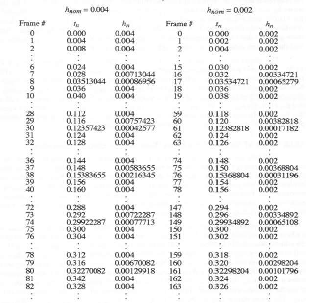
In order to produce real-time outputs at frame times that are integer multiples of   from data points for which the solution differs from real time because  , it is necessary to use extrapolation. Here we employ quadratic extrapolation based on displacement position and velocity at the nth frame and position at the n – 1 frame. Thus the formula for the extrapolated output  at time   based on the simulation outputs   and   is given by

(11.65)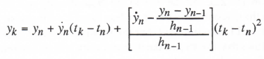 

 

An equivalent formula is used to obtain   from  ,   and  . For the simulation considered in this section, extrapolation is indeed required to compute the real-time outputs that fall within the integration frames involving steps to discontinuities. For example, in Table 11.1 for the case where   = 0.004, the real-time output   corresponding to   = 0.32 seconds is obtained using Eq. (11.65) with extrapolation based on Y and   for   = 0.28 and Y for   = 0.24. Similarly, real-time outputs for   = 0.120, 0.152, 0.296, 0.320, … also require extrapolation. Between these   values that require extrapolation, the discrete simulation output times   coincide exactly with the real-time data sequence times   and no extrapolation is necessary.

 

The output errors in simulating the two-dof system with friction are shown in Figure 11.26. The errors were determined by subtracting the reference solution with   = 0.000125 from the solutions with   = 0.002 and 0.004. Note that the errors shown in the figure have been normalized by dividing the actual errors in relative displacement Y and unsprung mass displacement Y2 by the amplitude A of the sinusoidal input of Eq. (11.64). Figure 11.26 shows that the errors for   = 0.004 are roughly four times the errors for   = 0.002. This confirms that the variable-step technique used here to handle the discontinuities caused by friction has preserved the   dependence of second-order predictor integration errors.

 

11.12. Effect of Increased Execution Time for the Step to Discontinuity

Until now we have assumed that every integration step in the simulation requires the same computer execution time, which was set equal to  , the nominal step size in the example simulation. On the other hand, it is evident that the equations which must be processed in order to implement the integration step that ends at a time of discontinuity will be likely to require more execution time than the routine, fixed-step AB-2 integrations. In this section we examine how such increased execution time can be handled in the simulation of our two-dof system with friction, and the corresponding effect on the simulation error.

 

Let us assume that the step to the discontinuity requires an execution time of  , where we have assumed until now that R =1 but just noted that R may in general exceed 1. In this case the scheme described in Section 11.7 and employed in the example simulation of Section 11.11 can still be used if we implement integration to the time of discontinuity whenever the step   required to do so becomes less than  .  This means that the step   to the discontinuity will then range between   and  , and it follows that the simulation outputs representing states at the time   of discontinuity will always be available ahead of real time. We can continue to use the quadratic extrapolation of Eq. (11.65) to calculate real-time outputs corresponding to  . The Euler startup step for the n + 1 frame will now be given by  , which as before will range between 0 and  , with the outputs at the end of the n+1 frame back on real time. The time corresponding to the end of the n + 1 frame is given by  .

 

The numerical example of Section 11.11 can again be used for illustration purposes. Assume that the execution time for each frame is 4 milliseconds, except for the frame involving the step to the discontinuity, which requires 10 milliseconds. In this case   is again equal to 4 milliseconds, but now R = 2.5, and the step to the discontinuity will be initiated whenever the time   required to reach the discontinuity becomes less than   or 14 milliseconds. As in the example of Section 11.11, assume next that the relative velocity Ydot reverses sign at t = 33.6 milliseconds. It follows that the step to the discontinuity will be implemented during the frame that begins at   =20 milliseconds, with the step size   equal to 13.6 milliseconds. The simulation result

 

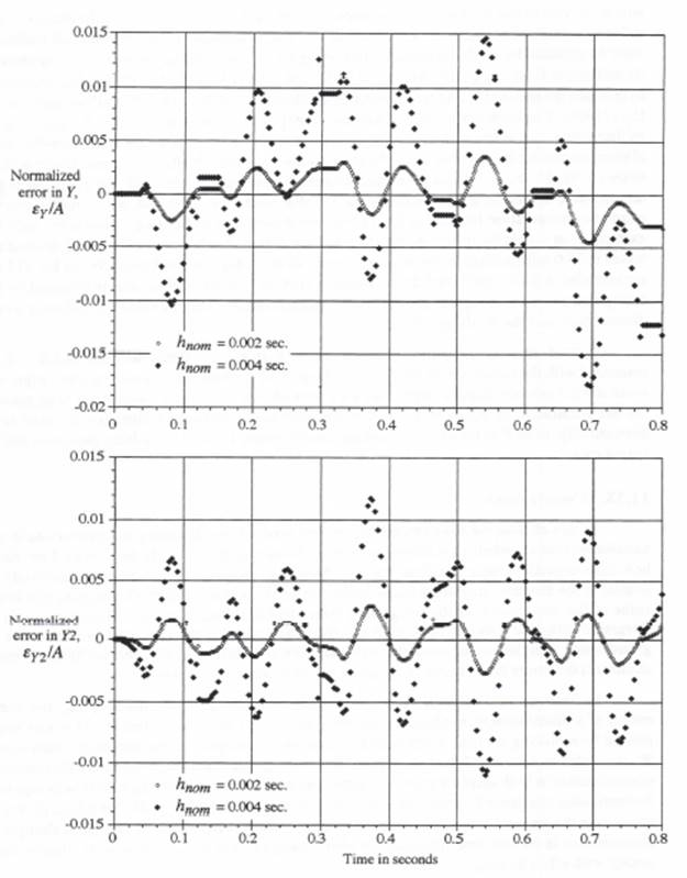
Figure 11.26.  Normalized simulation error in relative displacement Y and unspring mass displacement Y2 for nominal integration step sizes of 0.002 and 0.004 seconds

 

at the end of the nth frame will become available at t = 20 + 10 = 30 milliseconds, i.e., 3.6 milliseconds ahead of real time. The real time outputs corresponding to   = 24 and 28 milliseconds must be obtained by quadratic extrapolation using Eq. (11.65). When the real time outputs for   = 32 milliseconds are computed from Eq. (11.65), the results actually represent interpolation, since in this case the states at   = 33.6 milliseconds are already available at   = 32 milliseconds for use in Eq. (11.65). The Euler startup frame will have a step size given by   milliseconds, and at the end of this frame, i.e., at   + 2 = 33.6 + 0.4 = 34 milliseconds, the simulation outputs are back on real time. Note that the subsequent simulation outputs occur at discrete times t = 38, 42, 46, … milliseconds until the next discontinuity is reached. To continue to generate real-time outputs at integer multiples of 4 milliseconds, i.e., at 40, 44, 48, … milliseconds, the quadratic extrapolation formula of Eq. (11.65) must continue to be used. However, only linear extrapolation should be employed for the real-time output that follows the time of discontinuity, which is 33.6 milliseconds in our example here. In this case the quadratic term in Eq. (11.65) is not included in the formula, and the real-time output for   = 36 milliseconds is obtained by linear extrapolation based on   and   at t = 33.6 milliseconds. This avoids extrapolating over the discontinuity and the resulting large errors.

 

Actual simulation results for the above case with   = 0.004 seconds and R = 2.5 are compared with the earlier results for R = 1 in Figure 11.27. Note that the normalized output errors when R = 2.5 are only slightly larger than the errors when R = 1, even though it has been necessary for the simulation to adapt to a 150 percent increase in execution time for the step to each discontinuity, as well as the extensive extrapolation needed to fill the resulting gaps with real-time output data.

 

11.13. Conclusions

In this chapter we have considered several methods for handling discontinuities in state-variable derivatives when a simulation must be performed in real time. In Section 11.2 we showed how time-dependent input functions which exhibit step changes that occur asynchronously with respect to the discrete integration frame times can be accommodated by determining the average value of the step input over the integration frame within which it occurs. This average is then integrated using the Euler method, with any remaining terms in the state-variable derivative integrated using a higher-order predictor method. We demonstrated that this technique virtually eliminates the errors that are normally caused by asynchronous step inputs.

 

In Sections 11.3 through 11.6 we introduced a method for determining  , the average output of a discontinuous nonlinear function over a given integration frame. This was accomplished by replacing the time average by the average with respect to the nonlinear function input. We were able to derive analytic formulas for the resulting   function for nonlinearities containing discontinuities in both displacement and slope. As in the case of time-dependent step inputs, the discontinuous nonlinear function was integrated over each frame by multiplying  , its average value over the frame, by the integration step size. The effectiveness of the   technique was demonstrated in the real-time simulation of a bang-bang control system, as well as a linear control system with effort limiting.

 

In Sections 11.7 through 11.12 we considered the technique of handling discontinuities in dynamic systems by integrating directly to the time of occurrence for each discontinuity. We demonstrated how the technique can be made compatible with real-time simulation by using

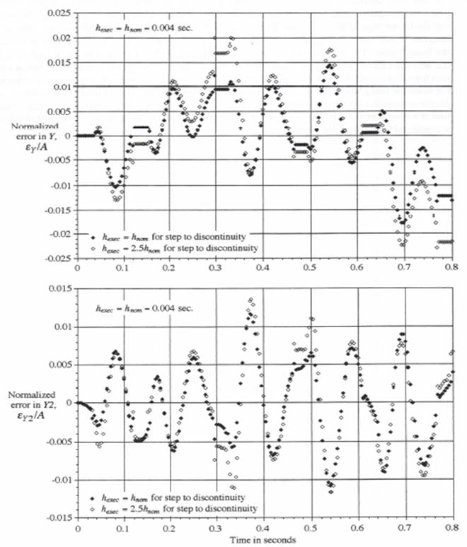
Figure 11.27. Comparison of normalized simulation errors with step-to-discontinuity execution times of  and 2.5  , where  = 0.004 seconds.

 

variable-step, second-order predictor integration. For any frame within which a discontinuity takes place, the integration step size is suitably increased from its normally fixed size of   in order to end the frame exactly at the time of discontinuity. For the first frame that follows, an Euler startup integration step less than   is utilized, so that the simulation is back on real time at the end of the Euler frame. This is followed by second-order predictor frames with fixed step size   until the next discontinuity is encountered. The technique can also handle the case where frame execution times for integration steps to discontinuities are significantly longer than frame execution times for nominal integration steps. Quadratic extrapolation has been shown to provide an accurate means to generate fixed-rate, real-time outputs from the variable-step simulation results. Simulation of a two-degree-of-freedom system with different levels of breakaway and running dry friction was utilized to illustrate the method.

 

Applied Dynamics International provides hardware, software, and engineering services for embedded software developers and control system engineers. Since 1957, ADI products have been used extensively in advanced control system applications in the aerospace, defense, training, and automotive industries. For more information on the complete ADI product family, please contact us at (734) 973-1300; email: adinfo@www.adi.com or visit our web site at www.adi.com. Dr. Howe is one of ADI’s founders and continues to the present as a Director and technical consultant.