10.1 Introduction
In this chapter we show how the real-time variable-step integration described in Chapter 9 can be combined with the multi-rate integration described in Chapter 8 to implement asynchronous real-time multi-rate simulation using either a single processor or multiple processors. Key to the successful implementation of both multi-rate integration and real-time variable-step integration is the use of accurate extrapolation formulas to convert data sequences from one frame rate to another, and to compensate for time mismatches and latencies in real-time data sequences. In both Chapters 8 and 9 we demonstrated that extrapolation based on the same algorithm used for numerical integration of the state equations can eliminate the data jitter and discontinuities so often associated with the use of more conventional extrapolation methods. In Chapter 8 we assumed that the frame-ratio N, i.e., the ratio of fast-to-slow integration frame rates in a multi-rate simulation, is always an integer. This has certainly been the choice in traditional multi-rate simulation. In this chapter we will show that multi-rate integration can be just as effective when the frame-ratio is not an integer, or indeed when the frame-ratio is not even fixed throughout a given simulation. Using the real-time variable-step predictor integration formulas introduced in Chapter 9, we will also show how processors engaged in real-time simulation can handle asynchronous interrupts without destroying the fidelity of the real-time simulation. Finally, we will demonstrate how the simulation of large complex dynamic systems can be partitioned among multiple processors, with each processor assigned to simulate identifiable physical subsystems. In this scheme each processor runs at its own frame rate, independent of the other processors, and data transfers between processors are handled with extrapolation algorithms similar to those developed in Chapters 8 and 9. Utilization of this asynchronous methodology has the potential of greatly reducing the difficulties usually associated with interconnecting many processors and hardware subsystems in a complex hardware-in-the-loop simulation.
We begin the chapter by showing how the real-time multi-rate simulation described in Chapter 8 can be modified to handle an increase in computer execution time within any given integration frame, such as might occur when an external interrupt must be processed. Later in the chapter we will show how the variable-step integration and associated extrapolation techniques can be used in multi-processor, multi-rate simulation of a combined digital-continuous system.
10.2 Accommodating a One-time Increase in Step Execution Time for a Multi-rate Simulation with Real-time Inputs and Outputs
Consider again the flight control system shown in Figure 8.2 of Chapter 8. In Section 8.9 we examined multi-rate simulation of the system using AB-2 integration, with the actuator considered to be the fast subsystem and the airframe to be the slow subsystem. We assumed that the times required to execute one integration step of the actuator and airframe were given, respectively, by ![]() and
and ![]() seconds. For a multi-rate frame ratio given by N = 8, Eqs. (8.1) and (8.2) yield integration step sizes for the actuator and airframe that are given, respectively, by
seconds. For a multi-rate frame ratio given by N = 8, Eqs. (8.1) and (8.2) yield integration step sizes for the actuator and airframe that are given, respectively, by ![]() and
and ![]() . For these step sizes, the resulting errors in real-time airframe and actuator outputs for an acceleration-limited unit-step input are shown in Figures 8.16 and 8.17. In this example simulation, scheduling the execution of fast and slow integration steps was based on the earliest next-half-frame occurrence. Table 8.1 shows that extrapolation of the real-time inputs is required to calculate 3 out of each 8 input data points
. For these step sizes, the resulting errors in real-time airframe and actuator outputs for an acceleration-limited unit-step input are shown in Figures 8.16 and 8.17. In this example simulation, scheduling the execution of fast and slow integration steps was based on the earliest next-half-frame occurrence. Table 8.1 shows that extrapolation of the real-time inputs is required to calculate 3 out of each 8 input data points ![]() for the actuator simulation. Also, extrapolation is needed in the calculation of 3 out of each 8 real-time actuator output data points
for the actuator simulation. Also, extrapolation is needed in the calculation of 3 out of each 8 real-time actuator output data points ![]()
In this section we consider the case where, every so often, the execution time for an individual integration step may increase substantially from time to time. For example, this might occur when complex conditional code must occasionally be implemented within a particular integration step. Or perhaps it may be desirable to have the capability of servicing an external interrupt now and then in the real-time simulation. For the multi-rate simulation in Section 8.9 we chose the integration step sizes ![]() and
and ![]() based on fixed and known step-execution times such that the real-time simulation always runs at maximum possible speed. Under these conditions, any increase in the execution time for a single integration step will cause the overall simulation to fall permanently behind real time by the amount of the execution-time increase. In this section we will introduce a methodology which lets the real-time simulation run at maximum possible speed when step-execution times are fixed, and yet permits occasional increases in step-execution time without compromising real-time simulation accuracy.
based on fixed and known step-execution times such that the real-time simulation always runs at maximum possible speed. Under these conditions, any increase in the execution time for a single integration step will cause the overall simulation to fall permanently behind real time by the amount of the execution-time increase. In this section we will introduce a methodology which lets the real-time simulation run at maximum possible speed when step-execution times are fixed, and yet permits occasional increases in step-execution time without compromising real-time simulation accuracy.
First, let us assume that the overall time, ![]() , required to execute N actuator steps followed by 1 airframe step is measured on-line using either the computer clock or master clock which controls the real-time simulation. For our multi-rate flight-control system simulation example with frame-ratio N = 8, let us further assume that the measurement of
, required to execute N actuator steps followed by 1 airframe step is measured on-line using either the computer clock or master clock which controls the real-time simulation. For our multi-rate flight-control system simulation example with frame-ratio N = 8, let us further assume that the measurement of ![]() is made just prior to executing the airframe integration formulas, i.e., just after the calculation of the airframe state-variable derivatives for the nth airframe step. Then
is made just prior to executing the airframe integration formulas, i.e., just after the calculation of the airframe state-variable derivatives for the nth airframe step. Then ![]() , represents the time required to execute the airframe integration formulas for the previous (n – 1) airframe step plus the following N actuator steps plus the state-variable derivative calculations for the nth airframe step. If the integration step-size
, represents the time required to execute the airframe integration formulas for the previous (n – 1) airframe step plus the following N actuator steps plus the state-variable derivative calculations for the nth airframe step. If the integration step-size ![]() used in the airframe integration formulas is then set equal to
used in the airframe integration formulas is then set equal to ![]() , and the integration step-size
, and the integration step-size ![]() used for the N following actuator steps is set equal to
used for the N following actuator steps is set equal to ![]() , the overall simulation will catch up with and remain synchronized with real time. By making the measurement of total execution time for N actuator steps plus 1 airframe step just prior to implementing the airframe integration formulas, we permit the airframe step size
, the overall simulation will catch up with and remain synchronized with real time. By making the measurement of total execution time for N actuator steps plus 1 airframe step just prior to implementing the airframe integration formulas, we permit the airframe step size ![]() for that very same step to be adjusted to reflect any change in execution time, instead of having to wait for the next (n + 1) airframe step. Note that any increase in airframe-step execution time, such as might result from required execution of conditional code, is more likely to occur in the derivative section of the nth airframe step. If we further require that external interrupts only be allowed in the derivative section of the airframe step, it follows that the correction in airframe step-size needed to handle either contingency in a real-time environment can still be accomplished within the nth airframe step.
for that very same step to be adjusted to reflect any change in execution time, instead of having to wait for the next (n + 1) airframe step. Note that any increase in airframe-step execution time, such as might result from required execution of conditional code, is more likely to occur in the derivative section of the nth airframe step. If we further require that external interrupts only be allowed in the derivative section of the airframe step, it follows that the correction in airframe step-size needed to handle either contingency in a real-time environment can still be accomplished within the nth airframe step.
As a specific example, suppose we let the execution time for one particular airframe integration step be doubled, from ![]() to
to ![]() seconds. For all other airframe integration steps we let
seconds. For all other airframe integration steps we let ![]() remain equal to its nominal value of 0.01. Also, we let the actuator integration step-execution time
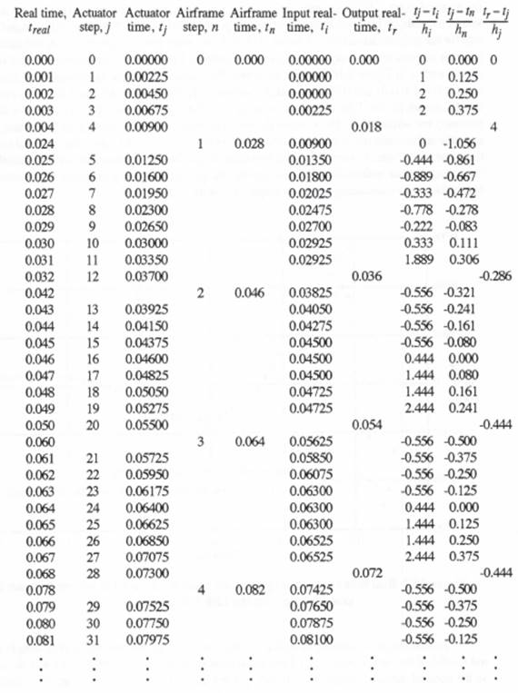
remain equal to its nominal value of 0.01. Also, we let the actuator integration step-execution time ![]() always remain equal to its nominal value of 0.001. Figure 10.1 shows the resulting timing diagram which, as in the earlier timing diagram of Figure 8.14, shows real time along the horizontal axis and mathematical simulation time (positive downward) along the vertical axis. The timing diagram of Figure 10.1 begins 4 actuator steps prior to the initiation of the 1st airframe step. Thus the first 4 actuator steps (j = 1, 2, 3, 4) in Figure 10.1 are
always remain equal to its nominal value of 0.001. Figure 10.1 shows the resulting timing diagram which, as in the earlier timing diagram of Figure 8.14, shows real time along the horizontal axis and mathematical simulation time (positive downward) along the vertical axis. The timing diagram of Figure 10.1 begins 4 actuator steps prior to the initiation of the 1st airframe step. Thus the first 4 actuator steps (j = 1, 2, 3, 4) in Figure 10.1 are
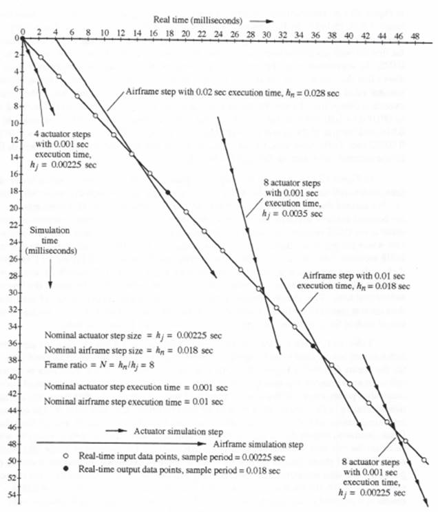
Figure 10.1. Timing diagram for real-time multi-rate simulation when the execution time for one airframe step is increased to 0.02 sec, then restored to 0.01 sec for follow-on steps.
the same as in Figure 8.14, where the 4th actuator step, representing ![]() , is completed after 0.004 seconds of real time. Then the first airframe step (n = 1) takes place, with a step-execution time of 0.02 seconds instead of the nominal value of 0.01. Thus the end of this first airframe step in Figure 10.1 occurs after 0.024 seconds of real time have elapsed. Because our measurement of
, is completed after 0.004 seconds of real time. Then the first airframe step (n = 1) takes place, with a step-execution time of 0.02 seconds instead of the nominal value of 0.01. Thus the end of this first airframe step in Figure 10.1 occurs after 0.024 seconds of real time have elapsed. Because our measurement of ![]() , which includes the 0.01 second increase in execution time of the airframe step, is by assumption made before implementing the airframe integration calculations, we are able to increase the first airframe integration step size in Figure 10.1 from the nominal size
, which includes the 0.01 second increase in execution time of the airframe step, is by assumption made before implementing the airframe integration calculations, we are able to increase the first airframe integration step size in Figure 10.1 from the nominal size ![]() to
to ![]() . In accordance with the methodology introduced in the above paragraph, Figure 10.1 shows that the step size for the next 8 actuator steps (j = 5, 6, … , 12) is increased from the nominal value of
. In accordance with the methodology introduced in the above paragraph, Figure 10.1 shows that the step size for the next 8 actuator steps (j = 5, 6, … , 12) is increased from the nominal value of ![]() to
to ![]() sec. Since the measured execution time of these 8 steps plus the next airframe step (n = 2) now returns to the nominal value of 8(0.001) + 0.01 = 0.018, the size of the 2nd airframe step in Figure 10.1 is returned to
sec. Since the measured execution time of these 8 steps plus the next airframe step (n = 2) now returns to the nominal value of 8(0.001) + 0.01 = 0.018, the size of the 2nd airframe step in Figure 10.1 is returned to ![]() , and the size of the next 8 actuator steps (j = 13, 14, …, 20) is returned to
, and the size of the next 8 actuator steps (j = 13, 14, …, 20) is returned to ![]() sec. In the same way, for all subsequent airframe and actuator steps,
sec. In the same way, for all subsequent airframe and actuator steps, ![]() remains 0.018 for the airframe and
remains 0.018 for the airframe and ![]() remains 0.00225 for the actuator.
remains 0.00225 for the actuator.
In Figure 10.1, as in the earlier timing diagram of Figure 8.14, events which occur in real time, such as real-time input samples ![]() , all lie on a straight line through the origin with slope of -1. We assume that real-time input samples continue to occur every 0.00225 seconds, i.e., with the nominal actuator step size, and that both real-time actuator and airframe outputs continue to occur every 0.018 seconds, i.e., with the nominal airframe step size. Later we will consider the case where the real-time actuator data points are required every 0.00225 seconds instead of every 0.018 seconds. The real-time input and output data points are shown in Figure 10.1 as light and dark circles, respectively, along the real-time line with slope -1. As in Figure 8.14, events which lie below this real-time line occur ahead of real time, and events which lie above the line occur behind real time. Thus the completion of the first 4 actuator steps occurs ahead of real time, as does the completion of the first airframe step. On the other hand, Figure 10.1 shows that completion of each of the next 6 actuator steps (j = 5,6, … , 10) occurs behind real time.
, all lie on a straight line through the origin with slope of -1. We assume that real-time input samples continue to occur every 0.00225 seconds, i.e., with the nominal actuator step size, and that both real-time actuator and airframe outputs continue to occur every 0.018 seconds, i.e., with the nominal airframe step size. Later we will consider the case where the real-time actuator data points are required every 0.00225 seconds instead of every 0.018 seconds. The real-time input and output data points are shown in Figure 10.1 as light and dark circles, respectively, along the real-time line with slope -1. As in Figure 8.14, events which lie below this real-time line occur ahead of real time, and events which lie above the line occur behind real time. Thus the completion of the first 4 actuator steps occurs ahead of real time, as does the completion of the first airframe step. On the other hand, Figure 10.1 shows that completion of each of the next 6 actuator steps (j = 5,6, … , 10) occurs behind real time.
Table 10.1, which is similar to the earlier Table 8.1 in Chapter 8, lists the actuator and airframe step indices j and n, the integration step times, ![]() and
and ![]() , and the associated real time,
, and the associated real time, ![]() , for the events depicted in Figure 10.1. Also shown in Table 10.1 is the input data-point time
, for the events depicted in Figure 10.1. Also shown in Table 10.1 is the input data-point time ![]() utilized at each actuator step-time
utilized at each actuator step-time ![]() , as well as the data-time
, as well as the data-time ![]() used in the calculation of real-time output data points every 0.018 seconds. Finally, Table 10.1 shows the dimensionless extrapolation interval,
used in the calculation of real-time output data points every 0.018 seconds. Finally, Table 10.1 shows the dimensionless extrapolation interval, ![]() , used to calculate each actuator real-time input data point
, used to calculate each actuator real-time input data point ![]() , the dimensionless extrapolation interval,
, the dimensionless extrapolation interval, ![]() , used to calculate the actuator inputs
, used to calculate the actuator inputs ![]() and
and ![]() from the airframe simulation outputs
from the airframe simulation outputs ![]() and
and ![]() , and the dimensionless extrapolation interval,
, and the dimensionless extrapolation interval, ![]() , used to calculate the real-time actuator output every 0.018 seconds. Comparison of Table 10.1 with the earlier Table 8.1 shows that the biggest increase in required extrapolation interval occurs in computing the real-time actuator output corresponding to
, used to calculate the real-time actuator output every 0.018 seconds. Comparison of Table 10.1 with the earlier Table 8.1 shows that the biggest increase in required extrapolation interval occurs in computing the real-time actuator output corresponding to ![]() (row 5, column 8). This is because when
(row 5, column 8). This is because when ![]() , the latest available actuator data point has the step time
, the latest available actuator data point has the step time ![]() . This results in a required extrapolation interval of 0.009, which corresponds to 4 actuator steps. The remaining extrapolation intervals listed in Table 10.1 are not very different from those shown earlier in Table 8.1. Note, however, that the increase from 0.01 to 0.02 in execution time for the first airframe step in Figure 10.1 and Table 10.1 results in a mismatch between real-time output sample times
. This results in a required extrapolation interval of 0.009, which corresponds to 4 actuator steps. The remaining extrapolation intervals listed in Table 10.1 are not very different from those shown earlier in Table 8.1. Note, however, that the increase from 0.01 to 0.02 in execution time for the first airframe step in Figure 10.1 and Table 10.1 results in a mismatch between real-time output sample times ![]() and both actuator and airframe simulation times
and both actuator and airframe simulation times ![]() and
and ![]() , respectively, for all follow-on steps. Thus the extrapolation interval for generating real-time actuator outputs every 0.018 seconds settles down to -0.444 actuator steps (equivalent to interpolation). This is evident in the last column of Table 10.1.
, respectively, for all follow-on steps. Thus the extrapolation interval for generating real-time actuator outputs every 0.018 seconds settles down to -0.444 actuator steps (equivalent to interpolation). This is evident in the last column of Table 10.1.
Table 10.1
Integration-step Indices, Step Times and Extrapolation Intervals for Multi-rate Simulation when the Execution Time for One Airframe Step is Increased to 0.02 Sec., Then Restored to 0.01 Sec. for Subsequent Steps; Frame-ratio N = 8.
10.3. Effect of Doubled Execution Time for the 12th Airframe Integration Step
We now let the one-time increase in airframe step-execution time occur in the 12th airframe integration step rather than the 1st integration step, as in Figure 10.1 and Table 10.1. As explained in the previous section, this means that the execution time for all the actuator steps is maintained at the nominal value of 0.001 seconds, the execution time for all airframe steps except the 12th is kept at 0.01 seconds, and the real-time output sample period is held at 0.018 seconds, the nominal step size for the airframe simulation. Figures 10.2 and 10.3 show the resulting errors in airframe and actuator outputs, respectively. Also shown in Figures 10.1 and 10.2 are the real-time output errors shown earlier in Figure 8.16 for the case where the execution time for all airframe and actuator steps is fixed at 0.01 and 0.001 seconds, respectively. In both Figures 10.2 and 10.3 it is evident that the errors for the first 11 output samples (i.e., for sample-times up to 11(0.018) = 0.198 seconds) are unchanged. Then, when the airframe execution time for step 12 is doubled, the airframe and actuator real-time output errors deviate from their original values for the fixed execution-time case. Note, however, that the deviation is significantly less than the errors themselves, indicating that our methodology for handling the change in airframe step-execution time, including extrapolation for maintaining real-time outputs, has worked effectively.
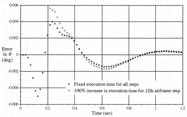
Figure 10.2. Real time airframe output errors resulting from a 100 percent increase in execution time for the 12th airframe step.
In addition to considering the actuator output errors when the real-time output sample period ![]() seconds, it is also useful to examine the errors when
seconds, it is also useful to examine the errors when ![]() , which is the same as the nominal actuator integration step size
, which is the same as the nominal actuator integration step size ![]() when the frame ratio N = 8. This has been done in
when the frame ratio N = 8. This has been done in
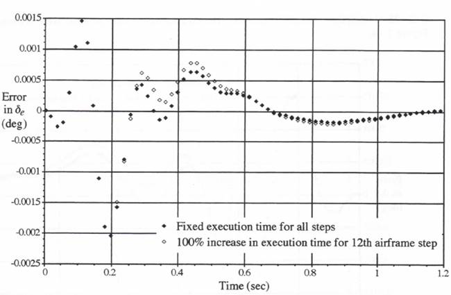
Figure 10.3. Real time actuator output errors resulting from a 100 percent increase in execution time for the 12th airframe step.
Figure 10.4, which shows the errors both with and without the increase from 0.01 to 0.02 in execution time for the 12th airframe step. Here we have reduced the length of displayed transient from 1.2 to 0.6 seconds in order to be able to distinguish better the individual error points. Note that the incremental errors associated with the much higher real-time output sample rate still remain small compared with the overall simulation errors.
Reference to row 5 in Table 10.1 shows that the maximum extrapolation interval ![]() required to generate real-time actuator outputs when
required to generate real-time actuator outputs when ![]() occurs during the airframe step with 0.02 second execution time. The actual extrapolation interval is equal to 0.018 – 0.009 = 0.009 seconds, which is equivalent to a dimensionless extrapolation interval
occurs during the airframe step with 0.02 second execution time. The actual extrapolation interval is equal to 0.018 – 0.009 = 0.009 seconds, which is equivalent to a dimensionless extrapolation interval ![]() , as shown in row 5 of the table. On the other hand, when the real-time output sample period
, as shown in row 5 of the table. On the other hand, when the real-time output sample period ![]() instead of 0.018, additional real-time outputs are required at
instead of 0.018, additional real-time outputs are required at ![]() , 0.02250 and 0.02475 seconds. The corresponding extrapolation intervals, based on
, 0.02250 and 0.02475 seconds. The corresponding extrapolation intervals, based on ![]() seconds for the 4th actuator step, are equal to 0.01125, 0.01350 and 0.01575, respectively. For the next real-time output at
seconds for the 4th actuator step, are equal to 0.01125, 0.01350 and 0.01575, respectively. For the next real-time output at ![]() seconds, row 7 in Table 10.1 shows that we can base the extrapolation on
seconds, row 7 in Table 10.1 shows that we can base the extrapolation on ![]() , since the next ( i.e., 5th) actuator step has been completed at
, since the next ( i.e., 5th) actuator step has been completed at ![]() . This reduces the required extrapolation interval to 0.0270 – 0.0195 = 0.0075. We conclude that the maximum extrapolation interval when computing real-time actuator outputs with
. This reduces the required extrapolation interval to 0.0270 – 0.0195 = 0.0075. We conclude that the maximum extrapolation interval when computing real-time actuator outputs with ![]() occurs when
occurs when ![]() and is equal to 0.01575. Note that this is considerably larger than the maximum extrapolation interval of 0.009 for the case where
and is equal to 0.01575. Note that this is considerably larger than the maximum extrapolation interval of 0.009 for the case where ![]() . In Figure 10.4, where the doubling of execution time occurs for the 12th instead of the 1st airframe integration step, the time
. In Figure 10.4, where the doubling of execution time occurs for the 12th instead of the 1st airframe integration step, the time ![]() associated with the maximum extrapolation interval of 0.01575 noted above, occurs at
associated with the maximum extrapolation interval of 0.01575 noted above, occurs at ![]() seconds. The corresponding extrapolation error is identified in Figure 10.4.
seconds. The corresponding extrapolation error is identified in Figure 10.4.
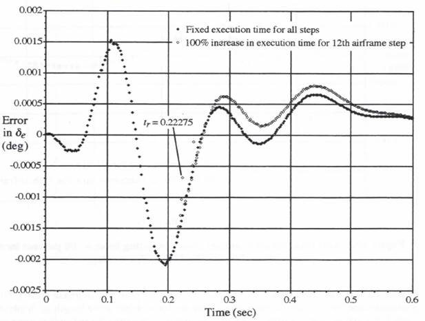
Figure 10.4. Real-time actuator output errors, sample-period = 0.00225, resulting from a 100 percent increase in execution time for the 12th airframe step.
It is useful to examine the local integration truncation errors when the execution time for the 12th airframe integration step is doubled. This has been done in Figure 10.5 for the airframe output ![]() and in Figure 10.6 for the actuator output
and in Figure 10.6 for the actuator output ![]() . Also shown in each figure is the local truncation error when the execution time for airframe step 12 is maintained at its nominal value of 0.01 second. In both cases the truncation error has been calculated on-line using the formula in Eq. (9.7). When
. Also shown in each figure is the local truncation error when the execution time for airframe step 12 is maintained at its nominal value of 0.01 second. In both cases the truncation error has been calculated on-line using the formula in Eq. (9.7). When ![]() is doubled from 0.01 to 0.02, the 0.01 second shift in discrete airframe step-time
is doubled from 0.01 to 0.02, the 0.01 second shift in discrete airframe step-time ![]() , that occurs for
, that occurs for ![]() is clearly evident in Figure 10.5.
is clearly evident in Figure 10.5.
Comparison of the local integration truncation errors shown in Figures 10.5 and 10.6 with the actual simulation errors in Figures 10.2 and 10.3, respectively, again demonstrates that local integration truncation errors can be used as an indicator of the effect of changes in integration step size on the overall simulation accuracy. In particular, we see in Figure 10.5 that the local truncation error associated with increasing the 12th airframe integration step size from 0.018 to 0.028 correlates directly with the increase in actual airframe output error shown in Figure 10.2. However, the airframe local truncation error increase in Figure 10.5 is confined almost entirely to
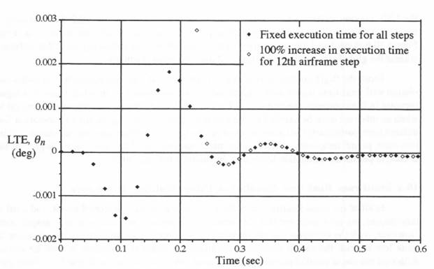
Figure 10.5. Local integration truncation error in real-time airframe output resulting from a 100 percent increase in execution time for the 12th airframe step.
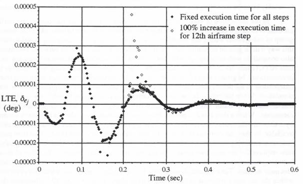
Figure 10.6. Local integration truncation error in real-time actuator output resulting from a 100 percent increase in execution time for the 12th airframe step.
the 12th integration step, whereas the global error increase in Figure 10.2 dies out only after a number of follow-on integration steps. Similarly, the actuator local truncation error increase in Figure 10.6 is confined almost entirely to the 8 actuator steps following the 12th airframe step, wheras the global error increase in Figure 12 dies out more gradually.
From the flight control system example considered here, we conclude that multi-rate simulation with real-time inputs and outputs can be accomplished even when there is a significant increase in the computer execution time for any particular integration step, such as might happen when an interrupt must be handled by the simulation computer. Again, the extrapolation formulas utilized here, particularly the formula based on the same algorithm used for the numerical integration itself, permit temporary increases in the mathematical size of the multi-rate integration steps, as needed to permit the simulation to once again catch up with real time.
10.4 Multi-rate Real-time Simulation Using Multiple Processors
In all of the considerations of multi-rate integration in Chapters 8 and 9, and until now in this chapter, we have assumed that the simulation is always implemented on a single computer. However, with the emergence in recent years of high-speed, single-chip microprocessors that are quite low in cost, the use of multiple computers for complex simulations must be considered. Although the use of parallel processors to improve overall computational speed has been a popular concept for many years, a good solution to the problem of efficiently distributing a large simulation among many processors has proven to be quite elusive. In particular, it has been difficult to partition the problem in such a way that the required number of data transfers between processors is minimized. Indeed, it has been the overhead associated with these data transfers that has invariably been the stumbling block in the efficient utilization of paralleled computer resources.
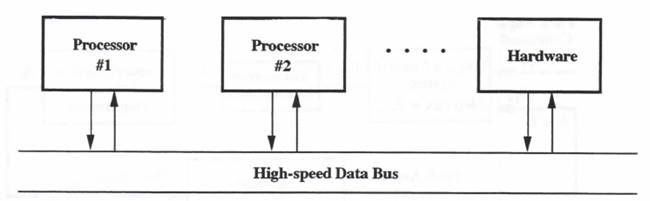
In the simulation of complex dynamic systems, one obvious solution to the partitioning problem is to assign each processor in a large simulation to an identifiable physical subsystem or group of subsystems within the overall system being simulated. Assigning multi-processors in this way will in general minimize the required number of data transfers between processors. It is also compatible with exchanging individual processor simulations with actual hardware, as in real-time HITL (hardware-in-the-loop) simulations. The problem of scheduling data transfers between processors can be greatly simplified by letting each processor or system run at its own frame rate, independent of the other frame rates. This is actually what we have designated here as multi-rate simulation. When the extrapolation methods introduced in Chapters 8 and 9 are used, it turns out that the individual frame rates no longer need to be integer multiples of each other, or even commensurate. When a data block is passed from one processor to another, it is always accompanied by a time-tag that identifies the discrete time represented by the data in that block and, when available, by the time derivatives of the variables contained in the data block. This then permits the processor receiving the data to reconstruct through extrapolation the value of each variable at the time required for use in its own simulation algorithm or physical process. Transfer of data blocks between processors and/or hardware subsystems can then be accomplished in a completely asynchronous manner. Time mismatches and data transfer delays can be automatically compensated to within the accuracy inherent in the extrapolation algorithms. Figure 10.7 illustrates the multiprocessor architecture in a real-time, hardware-in-the-loop simulation, as well as a data block with time tag and typical extrapolation formula.
Bus data: each data block consists of data values, their time derivatives (when available), and a time tag, i.e., ![]() . Then, using predictor-integration extrapolation
. Then, using predictor-integration extrapolation
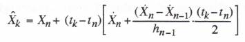
Figure 10.7. Multi-processor architecture.
In the sections that follow, we will describe how the asynchronous methodology can be applied to the multi-rate, multi-processor simulation of complex dynamic systems, with particular emphasis on real-time simulation with real-time inputs and outputs. The variable-step integration methods introduced in Chapter 9 will permit automatic assignment of integration frame rates within a given processor, as well as the ability to handle variable frame-execution times in an ongoing real-time simulation.
10.5 Example Simulation of a Mixed-data Flight Control System
To illustrate multi-processor simulation, we consider the airframe pitch control system shown in Figure 10.8. It consists of an airframe (the slow subsystem), a control-surface actuator (the fast subsystem), and a digital autopilot. The airframe is represented with the same mathematical model and system parameters used in the previous flight control system of Section 8.3. Thus the dynamic behavior of the airframe is dominated by the 5 rad/sec undamped natural frequency, ![]() , of the short-period pitching motion. Here the airframe will be simulated with a nominal integration step size of T = 0.02 seconds. The control-surface actuator is modeled as a second-order system with undamped natural frequency,
, of the short-period pitching motion. Here the airframe will be simulated with a nominal integration step size of T = 0.02 seconds. The control-surface actuator is modeled as a second-order system with undamped natural frequency, ![]() , equal to 40 rad/sec. It will be considered a fast subsystem, to be simulated with a nominal integration step size h = 0.005 seconds. The following control law is assumed for the digital controller:
, equal to 40 rad/sec. It will be considered a fast subsystem, to be simulated with a nominal integration step size h = 0.005 seconds. The following control law is assumed for the digital controller:
(10.1) ![]()
Here ![]() represents the digital controller output at the kth frame, K is the controller gain constant,
represents the digital controller output at the kth frame, K is the controller gain constant, ![]() is the input pitch angle, and
is the input pitch angle, and ![]() is the airframe output pitch angle at the kth frame, as generated by the A to D converter with sample-period
is the airframe output pitch angle at the kth frame, as generated by the A to D converter with sample-period ![]() . Also,
. Also, ![]() is the estimated pitch rate, as obtained from a backward difference approximation, and
is the estimated pitch rate, as obtained from a backward difference approximation, and ![]() is the effective rate constant.
is the effective rate constant.
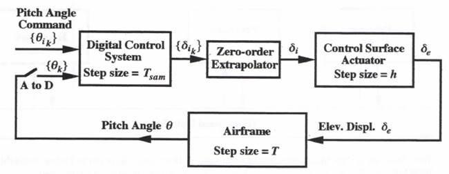
Figure 10.8. Block diagram of combined continuous/digital system simulation.
For illustrative purposes we select a digital controller frame rate of 100 Hz (i.e., ![]() seconds). The zero-order extrapolator in Figure 10.8 converts the output data sequence
seconds). The zero-order extrapolator in Figure 10.8 converts the output data sequence ![]() from the digital controller to the continuous input
from the digital controller to the continuous input ![]() for the control surface actuator. The actuator state equations take the form given earlier in Eq. (9.5), with X replaced by
for the control surface actuator. The actuator state equations take the form given earlier in Eq. (9.5), with X replaced by ![]() , Y replaced by
, Y replaced by ![]() , U(t) replaced by
, U(t) replaced by ![]() ,
, ![]() replaced by
replaced by ![]() , and
, and ![]() replaced by
replaced by ![]() . The following parameter values are used for the simulation:
. The following parameter values are used for the simulation:
![]()
For the sample-period given by ![]() for the digital controller and the above parameter values, the flight control system response to an acceleration-limited step input is shown in Figure 10.9. Here the solution was obtained using RK-4 integration with an integration step size h = T = 0.005, which is sufficiently small to ensure negligible dynamic errors. This solution serves as a reference for calculating simulation errors in the examples that follow.
for the digital controller and the above parameter values, the flight control system response to an acceleration-limited step input is shown in Figure 10.9. Here the solution was obtained using RK-4 integration with an integration step size h = T = 0.005, which is sufficiently small to ensure negligible dynamic errors. This solution serves as a reference for calculating simulation errors in the examples that follow.
With a nominal integration step size of T = 0.02 sec for the airframe simulation and h = 0.005 sec for the actuator simulation, the ratio between actuator and airframe integration frame rates in this case is given by N = 4. Since there are two actuator integration steps per digital controller step, i.e., ![]() , there is no problem in synchronizing the output samples of the zero-order extrapolator with the integration step times for the actuator simulation. Note, however, that the zero-order extrapolator will exhibit step changes in output every
, there is no problem in synchronizing the output samples of the zero-order extrapolator with the integration step times for the actuator simulation. Note, however, that the zero-order extrapolator will exhibit step changes in output every ![]() seconds as the extrapolator responds to each new digital controller output
seconds as the extrapolator responds to each new digital controller output ![]() . These steps become inputs to the actuator simulation, and large errors will result when the actuator is simulated using a standard predictor-integration method such as AB-2. To eliminate these errors we consider the actuator input
. These steps become inputs to the actuator simulation, and large errors will result when the actuator is simulated using a standard predictor-integration method such as AB-2. To eliminate these errors we consider the actuator input ![]() at the beginning of the jth frame to be representative of the input halfway through the frame, i.e.,
at the beginning of the jth frame to be representative of the input halfway through the frame, i.e., ![]() . The AB-2 difference equations for the actuator simulation with step size h then become the following:
. The AB-2 difference equations for the actuator simulation with step size h then become the following:
(10.2) ![]()
(10.3) ![]()
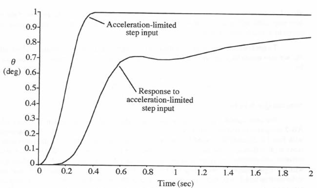
Figure 10.10. Control system response to acceleration-limited step input.
Note that the input term ![]() in Eq. (10.2) represents modified Euler integration with
in Eq. (10.2) represents modified Euler integration with ![]() , whereas the remaining terms on the right side of Eq. (10.2) represent AB-2 integration. In this way, accurate integration of the fixed input
, whereas the remaining terms on the right side of Eq. (10.2) represent AB-2 integration. In this way, accurate integration of the fixed input ![]() over the jth frame is achieved, without the problems normally suffered by predictor methods when discontinuous step inputs occur.
over the jth frame is achieved, without the problems normally suffered by predictor methods when discontinuous step inputs occur.
We recall that the same concept of mixing modified Euler integration with AB-2 integration was used earlier in Section 8.9 in simulating the airframe, where the airframe input ![]() was integrated using the modified Euler method and AB-2 integration was used for the remaining terms on the right side of Eq. (8.5). For a fixed airframe integration step size T, the airframe difference equations are then given by
was integrated using the modified Euler method and AB-2 integration was used for the remaining terms on the right side of Eq. (8.5). For a fixed airframe integration step size T, the airframe difference equations are then given by
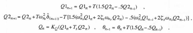
(10.4)
As in Section 8.9, the actuator output ![]() half-way through the nth airframe step is obtained using extrapolation based on the multi-rate actuator data points
half-way through the nth airframe step is obtained using extrapolation based on the multi-rate actuator data points ![]() and their time derivatives. By analogy with Eq. (8.14), the extrapolation formula is given by
and their time derivatives. By analogy with Eq. (8.14), the extrapolation formula is given by
(10.5) 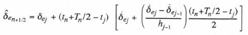
Here ![]() represents the nth airframe integration step size and
represents the nth airframe integration step size and ![]() represents the size of the n – 1 actuator step, although in our initial simulation example, both
represents the size of the n – 1 actuator step, although in our initial simulation example, both ![]() and
and ![]() will be constant step sizes given by T and h, respectively.
will be constant step sizes given by T and h, respectively.
To generate the controller input data point estimate ![]() from the airframe output data points
from the airframe output data points ![]() , we also use extrapolation based on second-order predictor integration. The formula is given by
, we also use extrapolation based on second-order predictor integration. The formula is given by
(10.6) 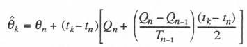
Note that ![]() in Eq. (10.6).
in Eq. (10.6).
We now consider the overall simulation of the flight control system in Figure 10.8 using AB-2 integration with fixed step size. The difference equations consist of (10.1) through (10.4), with Eqs. (10.5) and (10.6) used for the extrapolation required to interface the subsystem simulations with different frame rates. We will consider three cases. For the first case we set the airframe and actuator step sizes equal to their nominal values, T = 0.02 and h = 0.005, respectively, with the digital controller step size given by ![]() . For the second and third cases we let the airframe step size
. For the second and third cases we let the airframe step size ![]() , i.e., T = 0.022094 and 0.017906. These step sizes correspond to frame ratios between actuator and airframe step sizes given by N = 4.41888 and N = 3.58112, respectively, compared with the nominal frame ratio of N = 4. Figure 10.11 shows the error in simulated airframe output for the all three cases. Clearly the extrapolation formulas used to compensate for the non-commensurate frame ratios are quite effective, in that they produce incremental errors which are small compared with the basic errors associated with the finite integration
, i.e., T = 0.022094 and 0.017906. These step sizes correspond to frame ratios between actuator and airframe step sizes given by N = 4.41888 and N = 3.58112, respectively, compared with the nominal frame ratio of N = 4. Figure 10.11 shows the error in simulated airframe output for the all three cases. Clearly the extrapolation formulas used to compensate for the non-commensurate frame ratios are quite effective, in that they produce incremental errors which are small compared with the basic errors associated with the finite integration
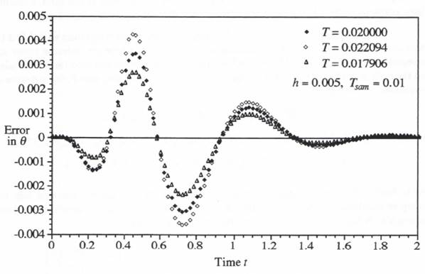
Figure 10.11. Effect of airframe simulation step size on error of simulated output.
step sizes used in the simulation. Indeed, the error differences for the three cases in Figure 10.11 can be entirely explained by the second-order truncation errors associated with each different step size T, as used in the airframe simulation.
We next consider the effect of varying the actuator simulation step size h from its nominal value of 0.005 sec. In this case the ratio of the digital-controller step size, ![]() , to the actuator step size h will no longer be 2:1. Therefore, we can no longer rely on the interpretation of
, to the actuator step size h will no longer be 2:1. Therefore, we can no longer rely on the interpretation of ![]() to represent
to represent ![]() , as in the
, as in the ![]() term in Eq. (10.2), to eliminate first-order errors. The problem is illustrated in Figure 10.12, which shows the controller sample times
term in Eq. (10.2), to eliminate first-order errors. The problem is illustrated in Figure 10.12, which shows the controller sample times ![]() , the controller output samples
, the controller output samples ![]() , the corresponding extrapolator output
, the corresponding extrapolator output ![]() , and the actuator frame times
, and the actuator frame times ![]() for the case where
for the case where ![]() and h = 0.0055 sec. Note that the extrapolator output sample
and h = 0.0055 sec. Note that the extrapolator output sample ![]() at the time
at the time ![]() is not representative of the extrapolator output over the entire jth step when the extrapolator output jumps to a new value before the step is completed. The problem is solved by actually computing the average extrapolator output over each actuator simulation time step using the following simple formula:
is not representative of the extrapolator output over the entire jth step when the extrapolator output jumps to a new value before the step is completed. The problem is solved by actually computing the average extrapolator output over each actuator simulation time step using the following simple formula:
(10.7) ![]()
The average extrapolator output over the jth actuator time step, ![]() is shown in Figure 10.13. This output then replaces the input
is shown in Figure 10.13. This output then replaces the input ![]() in the modified AB-2 integration algorithm of Eq. (10.2). Using this procedure, we obtain the results in Figure 10.14, where the error in simulated output is shown for three different actuator simulation step sizes. For the first step size, h = 0.005, its nominal value. For the second and third step sizes,
in the modified AB-2 integration algorithm of Eq. (10.2). Using this procedure, we obtain the results in Figure 10.14, where the error in simulated output is shown for three different actuator simulation step sizes. For the first step size, h = 0.005, its nominal value. For the second and third step sizes, ![]() , i.e., h = 0.0060472, and 0.0039528. Note that the change in step size h has very little effect on the simulation, which indicates that the use of Eq. (10.7) to compensate for the non-integer ratio
, i.e., h = 0.0060472, and 0.0039528. Note that the change in step size h has very little effect on the simulation, which indicates that the use of Eq. (10.7) to compensate for the non-integer ratio ![]() that occurs when h = 0.0060472 and 0.0039528 is indeed very effective.
that occurs when h = 0.0060472 and 0.0039528 is indeed very effective.
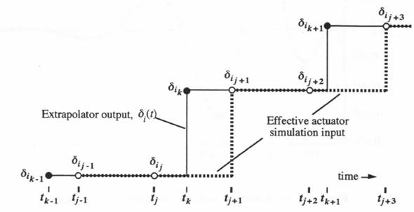
Figure 10.12. Extrapolator output and effective actuator input for a non-integer frame-rate ratio.
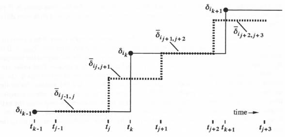
Figure 10.13. Extrapolator output and effective actuator input based on input averaging for a non-integer frame-rate ratio.
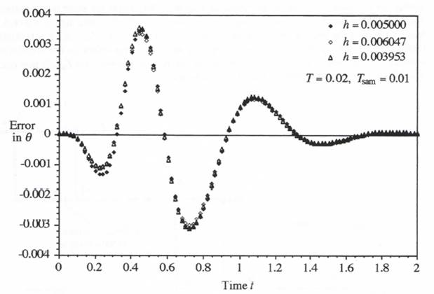
Figure 10.14. Effect of varying the actuator step size h.
Next, with the actuator step size fixed at the nominal value h = 0.005 and the digital controller step size still set to ![]() , we investigate the effectiveness of the variable-step second-order predictor integration method when used to simulate the airframe. The AB-2 difference equations for the airframe, given earlier in Eq. (10.4), must be modified in accordance with Eq. (9.2) to accommodate the variable airframe step size
, we investigate the effectiveness of the variable-step second-order predictor integration method when used to simulate the airframe. The AB-2 difference equations for the airframe, given earlier in Eq. (10.4), must be modified in accordance with Eq. (9.2) to accommodate the variable airframe step size ![]() . The difference equations for integrating the airframe state equations given in Eqs. (8.4) through (8.7) now become
. The difference equations for integrating the airframe state equations given in Eqs. (8.4) through (8.7) now become
(10.8) 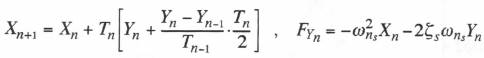
(10.9) 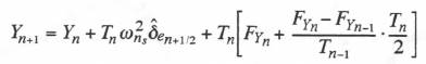
(10.10) 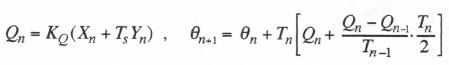
Note that the modified Euler input term ![]() on the right side of Eq. (10.9) is preserved in the variable-step predictor algorithm. Eq. (10.6) is used as before to produce the controller input data estimate
on the right side of Eq. (10.9) is preserved in the variable-step predictor algorithm. Eq. (10.6) is used as before to produce the controller input data estimate ![]() , as is Eq. (10.5) for the actuator output
, as is Eq. (10.5) for the actuator output ![]() halfway through the nth frame. Eqs. (10.1), (10.2), and (10.3) are also used as shown, with the exception that
halfway through the nth frame. Eqs. (10.1), (10.2), and (10.3) are also used as shown, with the exception that ![]() in Eq. (10.2) is again replaced by the mean value,
in Eq. (10.2) is again replaced by the mean value, ![]() of the extrapolator output over the jth frame, as given by Eq. (10.7).
of the extrapolator output over the jth frame, as given by Eq. (10.7).
As a specific example of a variable step size, we let the airframe integration step be given by ![]() . This represents the same relative variation is step size used earlier in our second-order system simulation and illustrated in Figure 9.1. Thus the airframe step size varies between 0.016 and 0.024 seconds, with a mean value of 0.02. Since the output of the airframe simulation will now exhibit a variable frame rate, with individual data points both behind and ahead of real time, we will use extrapolation based on second-order predictor integration to generate a fixed-step real-time output. We recall that this worked well in Section 9.3 in the variable-step simulation of the simple second-order system. The real-time extrapolation is accomplished by using Eq. (10.6), but with the digital controller time
. This represents the same relative variation is step size used earlier in our second-order system simulation and illustrated in Figure 9.1. Thus the airframe step size varies between 0.016 and 0.024 seconds, with a mean value of 0.02. Since the output of the airframe simulation will now exhibit a variable frame rate, with individual data points both behind and ahead of real time, we will use extrapolation based on second-order predictor integration to generate a fixed-step real-time output. We recall that this worked well in Section 9.3 in the variable-step simulation of the simple second-order system. The real-time extrapolation is accomplished by using Eq. (10.6), but with the digital controller time ![]() replaced by the fixed-step output time
replaced by the fixed-step output time ![]() . We let the step size of the real-time output data points be 0.02, the mean value of the variable step
. We let the step size of the real-time output data points be 0.02, the mean value of the variable step ![]() of the airframe simulation. Figure 10.15 shows the resulting airframe output errors in the variable-step case, as well as the output errors for a fixed airframe step size,
of the airframe simulation. Figure 10.15 shows the resulting airframe output errors in the variable-step case, as well as the output errors for a fixed airframe step size, ![]() (the mean of the variable-step size), and the errors when
(the mean of the variable-step size), and the errors when ![]() (the maximum value of the variable-step size). Note that the errors for the variable-step case are essentially the same as those for the fixed step when that step is equal to the mean variable-step size,
(the maximum value of the variable-step size). Note that the errors for the variable-step case are essentially the same as those for the fixed step when that step is equal to the mean variable-step size, ![]() . On the other hand, if the fixed step is set to accommodate the maximum variable step size,
. On the other hand, if the fixed step is set to accommodate the maximum variable step size, ![]() , the errors are significantly larger, i.e., by the ratio (0.024/0.02)2.
, the errors are significantly larger, i.e., by the ratio (0.024/0.02)2.
10.6 Multi-processor versus Single-processor Simulation
Until now we have tacitly assumed that our flight control system in Figure 10.8 is simulated using a single processor, even though each subsystem simulation employs a different frame rate (multi-rate integration). However, there may be times when it is desirable, or even necessary, to simulate each subsystem on a separate processor. For example, in hardware-in-the-loop simulation, where initially the entire simulation is accomplished using computers, it will be easier to substitute actual hardware for one of the subsystems if an individual processor has been assigned
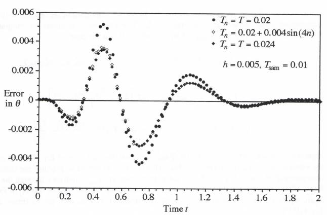
Figure 10.15. Output error for both fixed and variable airframe simulation steps.
for simulation of that subsystem. In this case the processor, including the appropriate interfacing, is simply replaced on a one-to-one basis with the hardware. Also, when the overall system being simulated is extremely complex, a single processor may be unable to handle the simulation with acceptable accuracy in real time, in which case multiple processors will be required. The simplest way of partitioning a large problem among parallel processors is to assign each processor to given physical subsystems or groups of subsystems. In this way the required number of data-variable transfers between processors, invariably the bottleneck in parallel-processor simulation, is likely to be minimized.
To illustrate, let us assume that three processors are assigned to the simulation of the flight control system in Figure 10.8, one for the digital controller, one for the zero-order extrapolator and control-surface actuator, and one for the airframe. In this case it makes particular sense to utilize variable-step integration based on the measured execution time of each integration frame in simulating the continuous subsystems (the actuator and airframe in our example here). The extrapolation formulas presented in Section 8.4 permit each processor to reconstruct the value of its input variables at the time required for use in its own simulation. This does mean that data-block transfers from one processor to another must include a time stamp that represents the discrete time associated with the block of data. Also, in order to implement extrapolation based on the same algorithm used to compute the output data by numerical integration, the time derivatives of each variable, when available, must also be included in the data-block transfers between processors.
The asynchronous multi-processor simulation using variable-step integration, as described in the above paragraph, can result in major simplifications of the programming task associated with data transfers in a complex, multi-processor simulation. It is instructive to examine a timing chart which shows frame execution times for the individual processors in a multi-rate, multi-processor simulation. For the nominal synchronous case where the controller step size ![]() , the actuator step size h = 0.005, and the airframe step size T = 0.02 seconds, this has been done in Figure 10.16a. Here we have assumed that the mathematical step size for each subsystem simulation has been set equal to the processor time required to execute that frame plus all input/output data transfers associated with the frame.
, the actuator step size h = 0.005, and the airframe step size T = 0.02 seconds, this has been done in Figure 10.16a. Here we have assumed that the mathematical step size for each subsystem simulation has been set equal to the processor time required to execute that frame plus all input/output data transfers associated with the frame.
For comparison purposes, Figure 10.16b shows the timing diagram when one processor is used for the entire simulation. In this latter case the single processor must be able to execute 1 airframe, 2 controller frames and 4 actuator frames in a total of 20 milliseconds in order for the simulation to run in real time. Also, in the single-processor program we must specify the order of execution of the different subsystem frames within each 20 millisecond total frame time. In Figure 10.16b we have chosen the frame-execution order based on the earliest next-full-frame occurrence for each subsystem. This was the first multi-rate scheduling algorithm described in Section 8.2 of Chapter 8. Thus at t = 0, the next actuator frame-end time (5 milliseconds) is the lowest, so that the actuator frame (marked Al in the figure) is the first to be executed. Starting at t = 5 milliseconds, the next frames for both the actuator (A2) and the controller (C1) end at t = 10 milliseconds. In Figure 10.16b we have assigned top priority to the controller, so that the first controller frame, Cl, is executed next. This is followed by the second and third actuator frames, A2 and A3. At the end of frame A3, the mathematical frame-end times for all three subsystems (frames A4, C2, and AF1) are equal to 20 milliseconds. Since the controller has the top priority, frame C2 is executed next, followed by A4 and finally AF1 (the lowest priority has been assigned to the airframe execution). In the synchronous case of Figure 10.16b, subsequent frame executions follow exactly the same order.
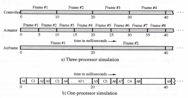
Figure 10.16. Timing diagram for one and three-processor multi-rate synchronous simulations; Tsam = 10, h = 5, T = 20 msec.
To illustrate an asynchronous case, we change the actuator step size h from 0.005 to 0.006047 seconds, with the controller and airframe step sizes retained at ![]() and T = 0.02 seconds, respectively. This is one of the cases shown earlier in Figure 10.14. The controller and airframe step sizes are now no longer commensurate with the actuator step size. The timing diagram for the three-processor simulation is shown in Figure 10.17a. Note that actuator frames no longer occur at exactly the same time as airframe or controller frames. Yet we have seen in Figure 10.14 that the extrapolation algorithms are able to compensate almost perfectly for the frame-time mismatches. In Figure 10.17b is shown the timing diagram for the single-processor simulation of the overall system. Here the order of frame executions is changed from that seen earlier in the synchronous case of Figure 10.16b. Thus frame AF1 for the airframe, instead of actuator frame A4, is executed after frame C2 for the controller. This is because the frame-end time for actuator frame A4 is now 24.189 milliseconds instead of 20 milliseconds, as in Figure 10.16b. Following frame AF1, the frame execution order in Figure 11.17b is A4, C3, A5, A6, C4, AF2, A7, … , instead of A5, C3, A6, A7, C4, A8, AF2, … , as shown earlier in the synchronous case of Figure 10.16b.
and T = 0.02 seconds, respectively. This is one of the cases shown earlier in Figure 10.14. The controller and airframe step sizes are now no longer commensurate with the actuator step size. The timing diagram for the three-processor simulation is shown in Figure 10.17a. Note that actuator frames no longer occur at exactly the same time as airframe or controller frames. Yet we have seen in Figure 10.14 that the extrapolation algorithms are able to compensate almost perfectly for the frame-time mismatches. In Figure 10.17b is shown the timing diagram for the single-processor simulation of the overall system. Here the order of frame executions is changed from that seen earlier in the synchronous case of Figure 10.16b. Thus frame AF1 for the airframe, instead of actuator frame A4, is executed after frame C2 for the controller. This is because the frame-end time for actuator frame A4 is now 24.189 milliseconds instead of 20 milliseconds, as in Figure 10.16b. Following frame AF1, the frame execution order in Figure 11.17b is A4, C3, A5, A6, C4, AF2, A7, … , instead of A5, C3, A6, A7, C4, A8, AF2, … , as shown earlier in the synchronous case of Figure 10.16b.
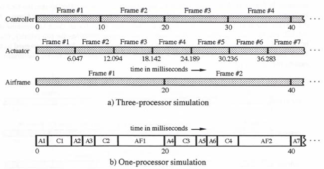
Figure 10.17. Timing diagram for one and three-processor multi-rate asynchronous simulations; Tsam = 10, h = 6.047, T = 20 msec.
In examining the multi-rate timing diagrams in Figures 10.16 and 10.17, it is important to consider Eq. (10.7), the formula used to compute ![]() , the average output of the zero-order extrapolator over the jth actuator frame. This formula requires
, the average output of the zero-order extrapolator over the jth actuator frame. This formula requires ![]() and
and ![]() , the extrapolator output at times
, the extrapolator output at times ![]() and
and ![]() , respectively. The determination of these outputs, in turn, requires knowledge of the digital controller output,
, respectively. The determination of these outputs, in turn, requires knowledge of the digital controller output, ![]() , for the controller frames which contain the times
, for the controller frames which contain the times ![]() and
and ![]() , respectively. For both the one and three-processor examples in Figures 10.16 and 10.17, it is readily apparent that this requirement is automatically satisfied.
, respectively. For both the one and three-processor examples in Figures 10.16 and 10.17, it is readily apparent that this requirement is automatically satisfied.
The above discussion of asynchronous multi-rate simulation has been directed to the real-time case. However, it should be noted that the methodology described here works equally well in the case of non-real-time simulation. Thus variable-step multi-rate simulation for general-purpose non real-time simulation can be accomplished in a very straightforward manner using the techniques introduced in this chapter. This, in turn, has the potential of providing substantial increases in computing efficiencies when simulating complex dynamic systems.
10.7 Extension of Multi-rate Asynchronous Methodology to Real-time Interfaces
In Chapter 5 we discussed the dynamics of digital-to-analog and analog-to digital conversion. This discussion included a description of algorithms to compensate for the dynamic errors associated with zero-order DAC’s, as well as the performance improvements that can be realized by using multi-rate digital-to-analog conversion. Also described in Chapter 5 were the advantages of using multi-rate input sampling and averaging in analog-to-digital conversion. It should be noted that the asynchronous, multi-rate methodology developed here in Chapter 10 can be applied equally well to D to A and A to D interface subsystems in a real-time simulation. Each interface subsystem is simply treated as another processor in the overall multi-processor environment. Thus data-block transfers into and out of interface subsystems are accompanied by time tags for the discrete data within the data block. This then allows complete asynchronous multi-rate operations using the appropriate extrapolation formulas. Also, any time delays, fixed or variable, that occur in the data transfers are automatically compensated to within the accuracies inherent in the extrapolation formulas.