9.1 Introduction
In the real time simulation of dynamic systems it has been traditional to use a fixed time step for numerical integration. Indeed, we have made this assumption in all of the previous chapters of these notes. As noted in Chapter 1, the overriding reason for not using a variable step size is the possibility that the mathematical step size can become smaller than the computer execution time for the calculations involved in a given integration frame. This in turn means that the simulation output at the end of that step will fall behind real time. Another reason for choosing a fixed time step in real-time simulation is the compatibility with fixed sample rates when dealing with real-time inputs and outputs. On the other hand, when conditional statements are present in the program that is executed every integration step, the frame execution time will not be constant. Also, the refresh operation associated with dynamic random-access memory will in general cause small variations in the execution time for each integration frame, as will the utilization of cache memory, depending on the frequency of cache “hits.” The mathematical step size in a fixed-step, real-time simulation must of necessity be set equal to the maximum expected value of the frame execution time, which often may not even be known in a complex simulation, in order to ensure the availability of simulation outputs in real time.
The argument given above for simulation using fixed-step integration based on the fixed sample-rate requirements for real-time inputs and outputs can be waived if we are willing to use the extrapolation methods described in both Chapters 4 and 8. In particular, the extrapolation formulas permit both real-time inputs and outputs to be corrected for any lack of synchronization with the computer-simulation frame times. This in turn allows variable-step integration methods to be employed for improved computational efficiency. It also permits the real-time computer simulation to be run with the mathematical step size for each successive integration step set equal to the measured execution time for the previous step. With this procedure, the simulation is always able to keep up with real time, at least to within a fraction of the integration step size. The procedure also permits the real-time integration step size to be set automatically by the software, without user intervention. On-line error estimates can be employed to alert the user if the simulation errors ever become excessively large.
In the following sections the formulas for real-time, variable-step second and third-order predictor integration are presented, as well as the formula for second-order predictor-corrector integration using a variable step. The effectiveness of the variable-step methods is then demonstrated using a second-order system as an example.
9.2 Variable-step, Second-order Predictor Integration
As we have noted in earlier chapters, the most widely used integration algorithm for real-time simulation has been the second-order Adams-Bashforth (AB-2) predictor method. Consider the following differential equation:
(9.1) 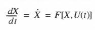
Here X is the state variable and U(t) is the explicit input function. In Chapter 8 we utilized Eq. (8.14) to achieve extrapolation based on second-order predictor integration. If we replace the extrapolation interval ![]() in Eq. (8.14) by the step size
in Eq. (8.14) by the step size ![]() for the nth integration step, and at the same time replace the step size
for the nth integration step, and at the same time replace the step size ![]() in Eq. (8.14) by the integration step size
in Eq. (8.14) by the integration step size ![]() for the
for the ![]() integration step, then in terms of the state X and its time derivative F, Eq. (8.14) becomes
integration step, then in terms of the state X and its time derivative F, Eq. (8.14) becomes
(9.2) 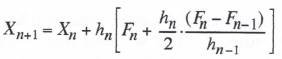
where
(9.3) ![]()
Here Eq. (9.2) represents the formula for variable-step, second-order predictor integration. For ![]() it reduces to the fixed-step AB-2 formula given by
it reduces to the fixed-step AB-2 formula given by ![]() . Note that the coefficient
. Note that the coefficient ![]() in Eq. (9.3) needs to be calculated only once each integration frame, regardless of the number of state variables being integrated. Eq. (9.2) then requires only 3 additions and 2 multiplications per state variable, compared with 2 additions and 2 multiplications in the case of fixed-step AB-2 integration. Thus the variable-step second-order predictor algorithm does not add significantly to the computational load when compared with fixed-step AB-2 integration. From the appropriate Taylor series expansions the following formula for the local truncation error associated with
in Eq. (9.3) needs to be calculated only once each integration frame, regardless of the number of state variables being integrated. Eq. (9.2) then requires only 3 additions and 2 multiplications per state variable, compared with 2 additions and 2 multiplications in the case of fixed-step AB-2 integration. Thus the variable-step second-order predictor algorithm does not add significantly to the computational load when compared with fixed-step AB-2 integration. From the appropriate Taylor series expansions the following formula for the local truncation error associated with ![]() can be derived:
can be derived:
(9.4) 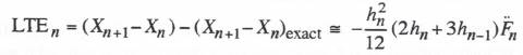
For ![]() the error reduces to the formula
the error reduces to the formula ![]() for fixed-step AB-2 integration.
for fixed-step AB-2 integration.
To illustrate the application of the variable-step second-order predictor algorithm, we consider the simulation of a linear second-order system with undamped natural frequency ![]() and damping ratio
and damping ratio ![]() . The state equations are given by
. The state equations are given by
(9.5) ![]()
Here X represents the output displacement, Y the output velocity, and U(t) the explicit input function. We let U(t) be the acceleration-limited unit step function defined earlier in Eq. (3.176). For ![]()
![]() and
and ![]() both the input U(t) and the system response X are plotted versus time t in Figure 3.14. From the figure it is evident that the solution X is very nearly the same as the response to an ideal unit step input that occurs at t = T. By using the acceleration-limited step input, we avoid the large transient errors inherent in predictor integration methods when subjected to discontinuous inputs. Also, the acceleration-limited input is more representative of inputs that are likely to occur in an actual dynamic system simulation.
both the input U(t) and the system response X are plotted versus time t in Figure 3.14. From the figure it is evident that the solution X is very nearly the same as the response to an ideal unit step input that occurs at t = T. By using the acceleration-limited step input, we avoid the large transient errors inherent in predictor integration methods when subjected to discontinuous inputs. Also, the acceleration-limited input is more representative of inputs that are likely to occur in an actual dynamic system simulation.
We now apply the variable-step predictor integration method to the simulation of the second-order system. In the integration formula of Eq. (9.2) we see from Eq. (9.5) that the derivative function ![]() in the formula for
in the formula for ![]() and that
and that ![]() in the formula for
in the formula for ![]() . We choose a nominal integration step size of h = 0.2, with the variable step size given by the formula
. We choose a nominal integration step size of h = 0.2, with the variable step size given by the formula ![]() . This results in the time-varying step size shown in Figure 8.1, which oscillates about 0.2 within the interval 0.16 to 0.24 and could be representative of the variable frame execution time in an actual simulation.
. This results in the time-varying step size shown in Figure 8.1, which oscillates about 0.2 within the interval 0.16 to 0.24 and could be representative of the variable frame execution time in an actual simulation.
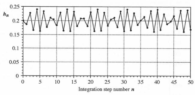
Figure 9.1. Variation in integration step size ![]() versus frame number n.
versus frame number n.
Using the variable-step predictor integration algorithm of Eq. (9.2) with the variable step size ![]() illustrated in Figure 9.1, we obtain the simulation results shown in Figure 9.2. Data points from the simulation are superimposed on the ideal response curve, shown earlier in Figure 3.14. The variation in step size
illustrated in Figure 9.1, we obtain the simulation results shown in Figure 9.2. Data points from the simulation are superimposed on the ideal response curve, shown earlier in Figure 3.14. The variation in step size ![]() is evident in the uneven time-axis spacing of the data points in Figure 9.2.
is evident in the uneven time-axis spacing of the data points in Figure 9.2.
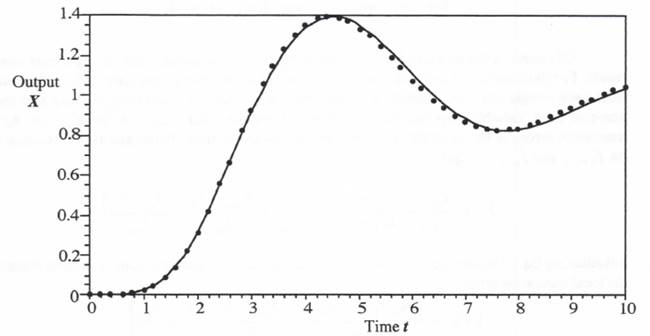
Figure 9. Simulated response using second-order predictor integration for the variable integration step size shown in Figure 9.1.
The accuracy of the simulation is easier to see in Figure 9.3, where the simulation error is plotted directly, along with the error when using a fixed step size of h = 0.2 (the mean value of the variable step size) and h = 0.24 (the maximum value of the variable step size). Note that the errors for the variable-step case are essentially the same as those for the fixed step when that step is equal to the mean, h = 0.2. On the other hand, if the fixed step is set to accommodate the maximum variable step size, h =0.24 and the errors are significantly larger, i.e., by the ratio (0.24/0.2)2.
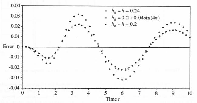
Figure 9.3. Error in simulated response using second-order predictor integration for both variable and fixed step sizes.
Of course, if the step size becomes much larger than the mean value, a significant error can result. For this reason it is desirable to be able to calculate on-line an estimate of the error resulting from each integration step. Indeed, such an estimate is a basis for selecting the step size itself in non-real-time, variable-step integration methods. Here we utilize Eq. (9.4) to calculate the local truncation error. In this formula, ![]() is determined using a central difference approximation based on
is determined using a central difference approximation based on ![]() and
and ![]() . Thus
. Thus
(9.6) 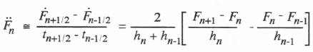
Substituting Eq. (9.6) into Eq. (9.4), we obtain the following numerical approximation formula for the local truncation error:
(9.7) 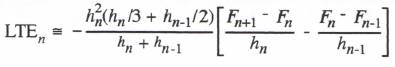
In this formula, the term ![]() will already need to have been computed to implement Eq. (9.2) for the n + 1 integration frame.
will already need to have been computed to implement Eq. (9.2) for the n + 1 integration frame. ![]() can be calculated by multiplying
can be calculated by multiplying ![]() by
by ![]() .
.
This same calculation will already have been performed for the nth frame, so that the calculation of local truncation error in Eq. (9.7) requires only 1 addition and 2 multiplications per state variable, once the coefficient ![]() has been computed for the n + 1 frame.
has been computed for the n + 1 frame.
In Figure 9.4 the local truncation error, as calculated for our example simulation using Eq. (9.7), is shown. Also shown for comparison is an exact calculation of the local truncation error. Here the exact local truncation error associated with ![]() is determined by computing the exact solution,
is determined by computing the exact solution, ![]() at
at ![]() , starting with the initial conditions
, starting with the initial conditions ![]() ,
, ![]() for the numerical solution at
for the numerical solution at ![]() . From Figure 9.4 it is evident that the numerical calculation agrees quite well with the exact calculation. Also evident in the figure is the substantial variation in local truncation error from step to step due to the variation in integration step size, as shown in Figure 9.1. For the second-order predictor integration method used here, we note that the local truncation error is proportional to the cube of the step size. It seems clear that an on-line numerical calculation of local truncation error can be relied upon to flag an unacceptable error resulting from too large a mathematical step size. When this occurs, the only recourse is to utilize a faster real-time computer or, in the case of a large simulation, to partition the simulation among several computers.
. From Figure 9.4 it is evident that the numerical calculation agrees quite well with the exact calculation. Also evident in the figure is the substantial variation in local truncation error from step to step due to the variation in integration step size, as shown in Figure 9.1. For the second-order predictor integration method used here, we note that the local truncation error is proportional to the cube of the step size. It seems clear that an on-line numerical calculation of local truncation error can be relied upon to flag an unacceptable error resulting from too large a mathematical step size. When this occurs, the only recourse is to utilize a faster real-time computer or, in the case of a large simulation, to partition the simulation among several computers.
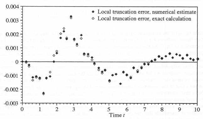
Figure 9.4. Local truncation error; numerical and exact calculations.
9.3 Use of Extrapolation to Produce a Fixed Frame-rate Output
In Figures 9.2 and 9.3 we have shown the simulation output and output error using data points that are unequally spaced in time as a result of the variable-step simulation. In general, not all of these output data points will be available in real time. In particular, if we set the mathematical step size in a real-time simulation equal to the measured execution time for the previous step, this causes the mathematical step size to be one step behind the actual measured execution time for each step. Furthermore, the output data sequence in a real-time simulation is often required at equally- spaced time intervals. For these reasons it is important to consider methods for reconstructing a fixed-rate, real-time output data sequence using extrapolation and/or interpolation. Actually, the same type of problem arises in the multi-rate simulation described in Chapter 8, where we must construct data sequences with one sample rate from data sequences with a different sample rate. In Section 8.4 we noted that this could be accomplished using linear extrapolation, as in Eqs. (8.12) or (8.13), with Eq. (8.13) preferred when the time derivative is directly available. In either case the extrapolation error is proportional to the square of the extrapolation interval. We also found in Chapter 8 that the most effective extrapolation algorithm is one based on the same algorithm used for integrating the state equations in the simualtion. This turns out to be Eq. (8.14) when AB-2 integration is used. In this case the extrapolation error is proportional to the cube of the extrapolation interval. When the time derivative of the variable being extrapolated is not directly available, the quadratic extrapolation given by Eq. (8.17) can be used in order to provide extrapolation with the error proportional to the cube of the extrapolation interval.
Assume, for example, that an output data sequence ![]() is required in real time with a fixed sample period given by
is required in real time with a fixed sample period given by ![]() . Starting with a data sequence
. Starting with a data sequence ![]() with variable sample period
with variable sample period ![]() and time derivatives given by
and time derivatives given by ![]() , we obtain the following extrapolation formula based on the counterpart of the predictor-integration formula given in Eq. (8.14):
, we obtain the following extrapolation formula based on the counterpart of the predictor-integration formula given in Eq. (8.14):
(9.8) 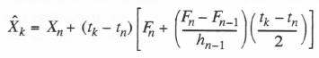
Here ![]() is the extrapolation interval which, when equal to the step size
is the extrapolation interval which, when equal to the step size ![]() , for the nth integration frame, reduces Eq. (9.8) to the variable-step integration formula in Eq. (9.2). In the implementation of Eq. (9.8), the most recently available data points
, for the nth integration frame, reduces Eq. (9.8) to the variable-step integration formula in Eq. (9.2). In the implementation of Eq. (9.8), the most recently available data points ![]() and
and ![]() are utilized. For the ± 20 percent variation in step size shown in Figure 9.1 for our example variable-step simulation, this can result in a substantial variation in the extrapolation interval needed to generate the fixed-step, real-time output data points
are utilized. For the ± 20 percent variation in step size shown in Figure 9.1 for our example variable-step simulation, this can result in a substantial variation in the extrapolation interval needed to generate the fixed-step, real-time output data points ![]() from the variable-step simulation output data points
from the variable-step simulation output data points ![]() . For example, suppose we let the sample-period
. For example, suppose we let the sample-period ![]() for the real-time, fixed-step output be equal to the mean value of the variable-step size
for the real-time, fixed-step output be equal to the mean value of the variable-step size ![]() , which from Figure 9.1 is equal to 0.2. Then Figure 9.5 shows a plot of the required extrapolation interval
, which from Figure 9.1 is equal to 0.2. Then Figure 9.5 shows a plot of the required extrapolation interval ![]() versus
versus ![]() for the first 50 integration steps. Note that whenever a simulation output
for the first 50 integration steps. Note that whenever a simulation output ![]() is generated behind real time, the dimensionless extrapolation interval equals or exceeds the mean integration-step size of 0.2. On the other hand, whenever a simulation output
is generated behind real time, the dimensionless extrapolation interval equals or exceeds the mean integration-step size of 0.2. On the other hand, whenever a simulation output ![]() occurs ahead of real time, the extrapolation interval is much smaller in magnitude than the mean integration step size, and can be either positive or negative. We have already noted that the formula given in Eq. (9.8) produces an extrapolated output that will exactly match the output later generated by numerical integration when the integration step size equals the extrapolation interval. Thus when
occurs ahead of real time, the extrapolation interval is much smaller in magnitude than the mean integration step size, and can be either positive or negative. We have already noted that the formula given in Eq. (9.8) produces an extrapolated output that will exactly match the output later generated by numerical integration when the integration step size equals the extrapolation interval. Thus when ![]() is at or close to 0.2 in Figure 9.5, the real-time outputs obtained by extrapolation will be very consistent with the simulation output data points. When the magnitude of
is at or close to 0.2 in Figure 9.5, the real-time outputs obtained by extrapolation will be very consistent with the simulation output data points. When the magnitude of ![]() in Figure 9.5 is small compared with 0.2, the extrapolation errors will of course also be quite small. In both cases this is quite evident in Figure 9.6, where the errors in real-time output
in Figure 9.5 is small compared with 0.2, the extrapolation errors will of course also be quite small. In both cases this is quite evident in Figure 9.6, where the errors in real-time output ![]() for
for ![]() are plotted along with the errors in the simulation output
are plotted along with the errors in the simulation output ![]() , when using the variable integration time steps shown in Figure 9.1 Figure 9.6 shows that the extrapolation performance is excellent, with real-time output extrapolation errors that are quite small compared with the simulation errors in general. We conclude that the use of Eq. (9.8) for extrapolation to produce real-time outputs is very effective.
, when using the variable integration time steps shown in Figure 9.1 Figure 9.6 shows that the extrapolation performance is excellent, with real-time output extrapolation errors that are quite small compared with the simulation errors in general. We conclude that the use of Eq. (9.8) for extrapolation to produce real-time outputs is very effective.
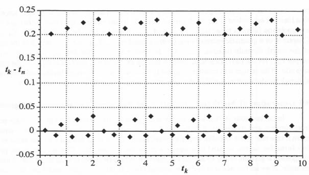
Figure 9.5. Extrapolation interval ![]() versus extrapolation time
versus extrapolation time ![]() .
.
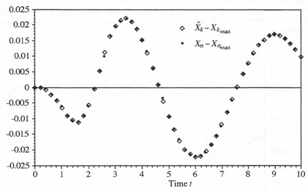
Figure 9.6. Errors in fixed-step output data points ![]() generated from variable-step points
generated from variable-step points ![]() using second-order predictor integration for extrapolation.
using second-order predictor integration for extrapolation.
Until now we have only considered the generation of real-time data points ![]() representing the output displacement in the variable-step simulation of the example second-order system. If it is necessary to provide fixed-rate, real-time output velocity data points
representing the output displacement in the variable-step simulation of the example second-order system. If it is necessary to provide fixed-rate, real-time output velocity data points ![]() the time derivative
the time derivative ![]() is not available at the beginning of the nth integration frame. Thus the predictor-integration extrapolation formula equivalent to Eq. (9.8) cannot be used. In this case we can resort either to a quadratic extrapolation formula based on
is not available at the beginning of the nth integration frame. Thus the predictor-integration extrapolation formula equivalent to Eq. (9.8) cannot be used. In this case we can resort either to a quadratic extrapolation formula based on ![]()
![]() and
and ![]() , which would be equivalent to Eq. (8.17) in Chapter 8, or a quadratic extrapolation formula based on
, which would be equivalent to Eq. (8.17) in Chapter 8, or a quadratic extrapolation formula based on ![]() ,
, ![]() and
and ![]() , which is the equivalent of the fourth formula listed in Table 4.1. In neither case will the formula match the simulation output
, which is the equivalent of the fourth formula listed in Table 4.1. In neither case will the formula match the simulation output ![]() for the next integration frame when the extrapolation interval is equal to the integration step size. This in turn will result in noticeably more scatter in the errors for the real-time output
for the next integration frame when the extrapolation interval is equal to the integration step size. This in turn will result in noticeably more scatter in the errors for the real-time output ![]() , although the data scatter is still likely to be small compared with the errors themselves.
, although the data scatter is still likely to be small compared with the errors themselves.
9.4 Generation of Multi-rate Outputs from Real-time Variable-step Integration
In the previous section we considered the generation of fixed-step real-time data points ![]() from variable-step data points
from variable-step data points ![]() when the frame rate
when the frame rate ![]() of the fixed-step output is equal to the mean frame rate of the variable step-size simulation. There is no reason why the same extrapolation formulas cannot be used to generate a multi-rate output
of the fixed-step output is equal to the mean frame rate of the variable step-size simulation. There is no reason why the same extrapolation formulas cannot be used to generate a multi-rate output ![]() . The second-order predictor-integration algorithm of Eq. (9.8) will be especially effective in generating multi-rate outputs. For example, if we let the step size
. The second-order predictor-integration algorithm of Eq. (9.8) will be especially effective in generating multi-rate outputs. For example, if we let the step size ![]() instead of 0.2 in our example simulation, the fixed frame rate
instead of 0.2 in our example simulation, the fixed frame rate ![]() of
of ![]() will be 2.5 times the mean frame rate of the variable-step simulation. Eq. (9.8) is again used to calculate
will be 2.5 times the mean frame rate of the variable-step simulation. Eq. (9.8) is again used to calculate ![]() , but it must now be implemented an average of 2.5 times per variable integration step
, but it must now be implemented an average of 2.5 times per variable integration step ![]() . Figure 9.7 shows the resulting errors in the multi-rate data points
. Figure 9.7 shows the resulting errors in the multi-rate data points ![]() as generated from the variable-step data points
as generated from the variable-step data points ![]() . As found previously in Figure 9.6, the extrapolation performance is excellent, with extrapolation errors quite small compared with the simulation errors in general.
. As found previously in Figure 9.6, the extrapolation performance is excellent, with extrapolation errors quite small compared with the simulation errors in general.
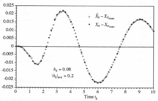
Figure 9.7. Errors in multi-rate output data points ![]() generated from variable-step data points
generated from variable-step data points ![]() , using second-order predictor integration for extrapolation.
, using second-order predictor integration for extrapolation.
9.5 Variable-step, Third-order Predictor Integration
In this section we consider variable-step third-order predictor integration (the fixed-step equivalent is AB-3 integration), which we will then apply to the same example real-time simulation considered thus far in this chapter. Third-order predictor integration has the advantage of improved accuracy, with global errors proportional to ![]() . It has the disadvantage of less robust stability than second-order predictor integration (see Figure 3.2). It also produces larger errors for discontinuous inputs. The formula for variable-step third-order predictor integration can be derived by following the same procedure used earlier in Section 8.12 to derive the third-order predictor-integration extrapolation formula of Eq. (8.24) for fixed integration steps. Thus we start with the following Taylor series approximation for
. It has the disadvantage of less robust stability than second-order predictor integration (see Figure 3.2). It also produces larger errors for discontinuous inputs. The formula for variable-step third-order predictor integration can be derived by following the same procedure used earlier in Section 8.12 to derive the third-order predictor-integration extrapolation formula of Eq. (8.24) for fixed integration steps. Thus we start with the following Taylor series approximation for ![]() using the state equation
using the state equation ![]() :
:
(9.9) 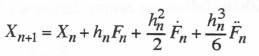
Central difference approximations for ![]() and
and ![]() of order
of order ![]() are given by the following formulas:
are given by the following formulas:
(9.10) 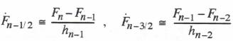
![]() is now represented to order h by a backward difference based on
is now represented to order h by a backward difference based on ![]() and
and ![]() . Thus
. Thus
(9.11) 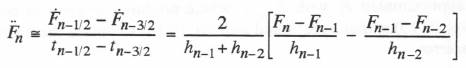
Note that this is equivalent to rewriting Eq. (9.6) for ![]() and then equating
and then equating ![]() to
to ![]() . To order
. To order ![]() , we can then write
, we can then write ![]() as
as
(9.12) 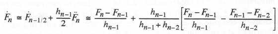
Substituting Eqs. (9.11) and (9.12) into (9.9), we obtain the following formula for third-order, variable-step predictor integration:
(9.13) 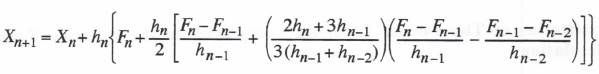
For ![]() , the formula reduces to
, the formula reduces to ![]() , which is just the standard AB-3 fixed-step integration formula first presented in Eq. (1.16). Also, comparison of Eq. (9.13) with Eqs. (9.2) and (9.7) shows that the first three terms on the right side of Eq. (9.13) represent the formula for second-order predictor integration, whereas the last term on the right side of Eq. (9.13) is simply the negative of the local truncation error,
, which is just the standard AB-3 fixed-step integration formula first presented in Eq. (1.16). Also, comparison of Eq. (9.13) with Eqs. (9.2) and (9.7) shows that the first three terms on the right side of Eq. (9.13) represent the formula for second-order predictor integration, whereas the last term on the right side of Eq. (9.13) is simply the negative of the local truncation error, ![]() , for second-order predictor integration. Note that the coefficients involving
, for second-order predictor integration. Note that the coefficients involving ![]() ,
, ![]() and
and ![]() in Eq. (9.13) need to be calculated only once per integration frame, regardless of the number of state variables to be integrated. Then each individual integration can begin with the calculation of
in Eq. (9.13) need to be calculated only once per integration frame, regardless of the number of state variables to be integrated. Then each individual integration can begin with the calculation of ![]() , which requires 1 addition and 1 multiplication by
, which requires 1 addition and 1 multiplication by ![]() . Since
. Since ![]() will have already been computed in the previous frame, completing the remaining calculations in Eq. (9.13) requires 4 additions and 3 multiplications. Thus implementation of the variable-step third-order integration formula of Eq. (9.13) is not as computationally intensive as it might first appear.
will have already been computed in the previous frame, completing the remaining calculations in Eq. (9.13) requires 4 additions and 3 multiplications. Thus implementation of the variable-step third-order integration formula of Eq. (9.13) is not as computationally intensive as it might first appear.
From Taylor series representations of ![]() ,
, ![]() and
and ![]() , the following formula for the local truncation error associated with third-order predictor integration can be derived:
, the following formula for the local truncation error associated with third-order predictor integration can be derived:

(9.14)
If it is necessary to calculate an estimate of the local truncation error at each integration step, then the required estimate of ![]() in Eq. (9.14) can be obtained by using the right side of Eq. (9.11) to represent a central-difference approximation for
in Eq. (9.14) can be obtained by using the right side of Eq. (9.11) to represent a central-difference approximation for ![]() , and an equivalent formula for
, and an equivalent formula for ![]() . Then we can approximate
. Then we can approximate ![]() with the following central difference formula based on
with the following central difference formula based on ![]() and
and ![]() :
:
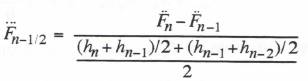
and
(9.15) 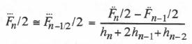
Here we have approximated ![]() with
with ![]() , which produces an error of order h due to the half-frame shift. Eqs. (9.15) is then substituted into Eq. (9.14) to obtain the formula for the estimated local truncation error.
, which produces an error of order h due to the half-frame shift. Eqs. (9.15) is then substituted into Eq. (9.14) to obtain the formula for the estimated local truncation error.
It should be noted that the calculation of local truncation error for the nth integration frame, whether we use either Eq. (9.7) for second-order predictor integration or Eq. (9.15) for third-order predictor integration, cannot be implemented until the n + 1 integration frame has been completed. For example, in Eq. (9.7) we see that ![]() must be available to compute
must be available to compute ![]() . Similarly,
. Similarly, ![]() must be available to compute
must be available to compute ![]() in Eq. (9.15). In both cases this results in a one-frame delay in the calculation of local truncation error. However, this one-frame delay is quite acceptable, since the error estimate itself is only used as an indicator of how large the simulation error may be due to an excessive integration step size.
in Eq. (9.15). In both cases this results in a one-frame delay in the calculation of local truncation error. However, this one-frame delay is quite acceptable, since the error estimate itself is only used as an indicator of how large the simulation error may be due to an excessive integration step size.
9.6 Application of Third-order Predictor Integration to the Example Variable-step Simulation
We now examine the performance of the variable-step, third-order predictor integration method when used to simulate the second-order system with an acceleration-limited unit-step input. Figure 9.8 presents plots of the error in simulated output ![]() for: (1) the variable step size illustrated in Figure 9.1, i.e.,
for: (1) the variable step size illustrated in Figure 9.1, i.e., ![]() ; (2) a fixed step
; (2) a fixed step ![]() (the mean value of the variable step size); (3) a fixed step
(the mean value of the variable step size); (3) a fixed step ![]() (the maximum value of the variable step size). We note that the errors for the variable step case are essentially the same as those for the fixed step when that step is equal to the mean, h = 0.2. This agrees with the results we found earlier in Figure 9.3 for second-order predictor integration. On the other hand, when the fixed step is set to accommodate the maximum variable step size, h = 0.24, the errors are significantly larger, i.e., by the ratio (0.24/0.2)3. This is because the third-order predictor integration used in Figure 18 exhibits global truncation errors proportional to the cube of the step size. We conclude that in the presence
(the maximum value of the variable step size). We note that the errors for the variable step case are essentially the same as those for the fixed step when that step is equal to the mean, h = 0.2. This agrees with the results we found earlier in Figure 9.3 for second-order predictor integration. On the other hand, when the fixed step is set to accommodate the maximum variable step size, h = 0.24, the errors are significantly larger, i.e., by the ratio (0.24/0.2)3. This is because the third-order predictor integration used in Figure 18 exhibits global truncation errors proportional to the cube of the step size. We conclude that in the presence
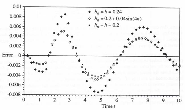
Figure 9.8. Error in simulated response using third-order predictor integration for both variable and fixed step sizes.
of a variable computer execution time for each integration step, there can be a significant accuracy improvement in using variable-step rather than fixed-step third-order predictor integration in real-time simulation. Note also that the output errors in Figure 9.8 are much smaller than those in Figure 93. This is to be expected, since the third-order method of Figure 9.8 exhibits global errors proportional to ![]() as opposed to
as opposed to ![]() for the second-order method of Figure 9.3, where
for the second-order method of Figure 9.3, where ![]() for
for ![]() and
and ![]() , as used in our example here.
, as used in our example here.
Next we consider the generation of a fixed-step, multi-rate output data sequence ![]() from the simulation output data sequence
from the simulation output data sequence ![]() as obtained here using variable-step, third-order predictor integration. In Section 9.3 we noted that extrapolation based on the same predictor algorithm used for the variable-step integration gives the best results. It has the further advantage of producing an extrapolated output
as obtained here using variable-step, third-order predictor integration. In Section 9.3 we noted that extrapolation based on the same predictor algorithm used for the variable-step integration gives the best results. It has the further advantage of producing an extrapolated output ![]() that exhibits errors,
that exhibits errors, ![]() , which are completely consistent with the variable-step output errors,
, which are completely consistent with the variable-step output errors, ![]() . This suggests that we should use third-order predictor integration for extrapolation to produce the fixed-rate data sequence
. This suggests that we should use third-order predictor integration for extrapolation to produce the fixed-rate data sequence ![]() from the variable-rate output data sequence
from the variable-rate output data sequence ![]() , in our example of this section. Thus Eq. (9.13) is used to compute
, in our example of this section. Thus Eq. (9.13) is used to compute ![]() , with the variable step
, with the variable step ![]() replaced by the extrapolation interval
replaced by the extrapolation interval ![]() . This leads directly to the following extrapolation formula:
. This leads directly to the following extrapolation formula:
(9.16) 
Here ![]() and
and ![]() are given in Eq. (9.10) and must be computed in any case to implement the variable-step integration algorithm. From Eq. (9.11),
are given in Eq. (9.10) and must be computed in any case to implement the variable-step integration algorithm. From Eq. (9.11), ![]() is given to order h by
is given to order h by
(9.17) 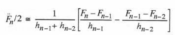
Again, this calculation will have already been made in implementing the variable-step integration algorithm. Once the coefficients ![]() and
and ![]() have been calculated, which requires 1 addition and 2 multiplications, the implementation of Eq. (9.16) for each extrapolation interval
have been calculated, which requires 1 addition and 2 multiplications, the implementation of Eq. (9.16) for each extrapolation interval ![]() requires 3 multiplications and 4 additions.
requires 3 multiplications and 4 additions.
As a specific example of fixed-step, multi-rate extrapolation, we examine the same case presented earlier in Section 9.4, where the fixed-step size ![]() is 0.08, compared with the mean size of 0.2 for the variable integration step
is 0.08, compared with the mean size of 0.2 for the variable integration step ![]() . This again results in a fixed frame rate
. This again results in a fixed frame rate ![]() for
for ![]() that is 2.5 times the mean frame rate of the variable-step simulation. It follows that Eq. (9.16) must be implemented an average of 2.5 times per variable integration step
that is 2.5 times the mean frame rate of the variable-step simulation. It follows that Eq. (9.16) must be implemented an average of 2.5 times per variable integration step ![]() . Figure 9.9 shows the resulting errors in the multi-rate data points
. Figure 9.9 shows the resulting errors in the multi-rate data points ![]() , as generated from the variable-step data points
, as generated from the variable-step data points ![]() , along with the errors in
, along with the errors in ![]() . As found previously in Figure 9.7 for second-order predictor integration, the extrapolation performance for third-order predictor integration is excellent, with the extrapolation errors quite small compared with the simulation errors in general.
. As found previously in Figure 9.7 for second-order predictor integration, the extrapolation performance for third-order predictor integration is excellent, with the extrapolation errors quite small compared with the simulation errors in general.
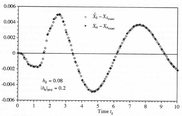
Figure 9.9. Errors in multi-rate output data points ![]() generated from variable-step data points
generated from variable-step data points ![]() using third-order predictor integration for extrapolation.
using third-order predictor integration for extrapolation.
9.7 Variable-step, Second-order Real-time Predictor-corrector Integration
Another candidate for real-time simulation using variable-step integration is the second-order predictor-corrector method, which we have previously designated as RTAM-2. In this two-pass algorithm the first pass through the state equations is used to compute an estimate ![]() of the state halfway through the step using second-order predictor integration. The formula is obtained directly from Eqs. (9.2) by replacing
of the state halfway through the step using second-order predictor integration. The formula is obtained directly from Eqs. (9.2) by replacing ![]() with
with ![]() . Thus we obtain
. Thus we obtain
(9.18) 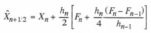
In the second pass through the state equations ![]() is used in the following formula to compute the derivative halfway through the integration step:
is used in the following formula to compute the derivative halfway through the integration step:
(9.19) ![]()
![]() is then used in the following modified Euler equation to calculate
is then used in the following modified Euler equation to calculate ![]() :
:
(9.20) ![]()
For this version of the second-order predictor-corrector method the local truncation error is given approximately by ![]() even in the variable-step case. This is 0.1 times the local truncation error associated with AB-2 integration for the same step size
even in the variable-step case. This is 0.1 times the local truncation error associated with AB-2 integration for the same step size ![]() . However, when one takes into account the dependence of global truncation error on
. However, when one takes into account the dependence of global truncation error on ![]() , it follows that the above two-pass predictor-corrector method will actually exhibit an asymptotic global accuracy that is 0.4 times that of the single-pass predictor method. This is because the two-pass method must, for a given processor operating in real time, utilize a mathematical step size which is twice that of a single-pass method. Using E.g. (9.17) to calculate
, it follows that the above two-pass predictor-corrector method will actually exhibit an asymptotic global accuracy that is 0.4 times that of the single-pass predictor method. This is because the two-pass method must, for a given processor operating in real time, utilize a mathematical step size which is twice that of a single-pass method. Using E.g. (9.17) to calculate ![]() , we can compute an on-line estimate of the local integration truncation error.
, we can compute an on-line estimate of the local integration truncation error.
To compare the predictor-corrector method introduced in this section with the predictor method used previously, we employ twice the variable step size utilized in the earlier predictor-integration examples. As noted above, this recognizes that it takes approximately twice as long per overall integration step for the execution of a two-pass method compared with a one-pass method. Thus we let ![]() in the fixed-step case and
in the fixed-step case and ![]() for the variable-step predictor-corrector simulation. The simulation results for both fixed and variable-step cases are presented in Figure 9.10. Also shown is the error for
for the variable-step predictor-corrector simulation. The simulation results for both fixed and variable-step cases are presented in Figure 9.10. Also shown is the error for ![]() , which represents a fixed step equal to the largest step size for the variable-step case. Comparison of the results with the errors obtained earlier in Figure 9.3 for predictor integration shows that the errors in Figure 9.10 for predictor-corrector integration are indeed smaller than those in Figure 9.3 for predictor integration. But the predictor-corrector errors are about 0.5 times the predictor errors, not 0.4 times, as expected based on the comparison of truncation errors in the above paragraph. This discrepancy is due to the relatively large nominal step size of 0.4 used in the predictor-corrector simulation. The validity of the approximate truncation error formulas is based on
, which represents a fixed step equal to the largest step size for the variable-step case. Comparison of the results with the errors obtained earlier in Figure 9.3 for predictor integration shows that the errors in Figure 9.10 for predictor-corrector integration are indeed smaller than those in Figure 9.3 for predictor integration. But the predictor-corrector errors are about 0.5 times the predictor errors, not 0.4 times, as expected based on the comparison of truncation errors in the above paragraph. This discrepancy is due to the relatively large nominal step size of 0.4 used in the predictor-corrector simulation. The validity of the approximate truncation error formulas is based on ![]() , which no longer applies when
, which no longer applies when ![]() and
and ![]() . For much smaller step sizes the predictor-corrector method will indeed produce errors which are 0.4 times those of the predictor method when using half the step size.
. For much smaller step sizes the predictor-corrector method will indeed produce errors which are 0.4 times those of the predictor method when using half the step size.
It is useful to examine the accuracy of the predictor estimate for ![]() , the integration output midway through each frame. For our example second-order system with the acceleration-limited step input, Figure 9.11 shows the errors in
, the integration output midway through each frame. For our example second-order system with the acceleration-limited step input, Figure 9.11 shows the errors in ![]() , as well as the errors in
, as well as the errors in ![]() , for the fixed-step case with
, for the fixed-step case with ![]() . From the figure it is apparent that the errors in
. From the figure it is apparent that the errors in ![]() are noticeably larger than the errors in
are noticeably larger than the errors in ![]() . This is not unexpected based on the local truncation error associated with the predictor algorithm of Eq. (9.18). From the appropriate Taylor series expansions it can be
. This is not unexpected based on the local truncation error associated with the predictor algorithm of Eq. (9.18). From the appropriate Taylor series expansions it can be
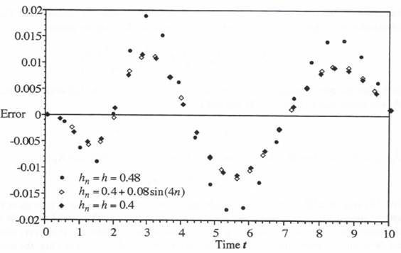
Figure 9.10. Error in simulated response using second-order predictor corrector integration for both variable and fixed step sizes.
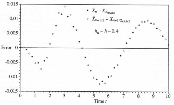
Figure 9.11. Simulation output errors at integer and half-integer frame times using predictor-corrector integration.
shown for the fixed-step case that the local truncation error in ![]() is given by
is given by ![]() , compared with the error
, compared with the error ![]() in
in ![]() for the corrector algorithm.
for the corrector algorithm.
When one examines the problem of determining suitable extrapolation formulas to produce accurate and smooth fixed-rate and multi-rate output data sequences ![]() from the variable-step predictor-corrector outputs
from the variable-step predictor-corrector outputs ![]() and their derivatives, it is not clear that a simple solution exists. Even in the case of fixed-step second-order predictor-corrector integration, we discussed at the end of Chapter 8 the difficulty in finding an extrapolation algorithm that does not exhibit discontinuities when the data upon which the extrapolation is based shifts from the predictor pass to the corrector pass and vice versa. This same problem continues to be present with all multiple-pass integration methods, including the Runge-Kutta algorithms. We therefore conclude that the single-pass predictor methods remain the most suitable algorithms for real-time simulation, as well as multi-rate simulation in general, when accurate extrapolation is required to generate data sequences that exhibit minimal discontinuities.
and their derivatives, it is not clear that a simple solution exists. Even in the case of fixed-step second-order predictor-corrector integration, we discussed at the end of Chapter 8 the difficulty in finding an extrapolation algorithm that does not exhibit discontinuities when the data upon which the extrapolation is based shifts from the predictor pass to the corrector pass and vice versa. This same problem continues to be present with all multiple-pass integration methods, including the Runge-Kutta algorithms. We therefore conclude that the single-pass predictor methods remain the most suitable algorithms for real-time simulation, as well as multi-rate simulation in general, when accurate extrapolation is required to generate data sequences that exhibit minimal discontinuities.
9.8. Input Extrapolation from Fixed-step to Variable-step Data Sequences
In all the examples considered thus far in this chapter, we have assumed that the exact input data sequence values ![]() have been available and are utilized for both fixed and variable-step simulations. The input data points may come from another dynamic simulation that uses either fixed or variable step sizes that are different from the step size
have been available and are utilized for both fixed and variable-step simulations. The input data points may come from another dynamic simulation that uses either fixed or variable step sizes that are different from the step size ![]() used in our example simulations here. In this case we must use extrapolation to calculate the proper input data points
used in our example simulations here. In this case we must use extrapolation to calculate the proper input data points ![]() . When this extrapolation is based on the same predictor integration method used to obtain U by numerical integration, we have seen that the resulting extrapolation errors become negligible. On the other hand, if U is derived from an external, real-time input, data points representing the time derivative
. When this extrapolation is based on the same predictor integration method used to obtain U by numerical integration, we have seen that the resulting extrapolation errors become negligible. On the other hand, if U is derived from an external, real-time input, data points representing the time derivative ![]() of the input will not in general be available. Furthermore, the resulting input data sequence is very likely to have a fixed sample period, which in many cases will be equal to the sample period
of the input will not in general be available. Furthermore, the resulting input data sequence is very likely to have a fixed sample period, which in many cases will be equal to the sample period ![]() of the required, real-time output data sequence. In this case the extrapolation formula for producing the variable-step input
of the required, real-time output data sequence. In this case the extrapolation formula for producing the variable-step input ![]() can only rely on current and past values of the fixed-step input data values
can only rely on current and past values of the fixed-step input data values ![]() .
.
For example, if we utilize an estimate for ![]() using linear extrapolation, then the extrapolation formula becomes
using linear extrapolation, then the extrapolation formula becomes
(9.21) 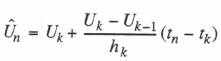
Here ![]() , corresponding to the real time
, corresponding to the real time ![]() , represents the most recent value of the input data sequence that is available when the calculation of the estimated input
, represents the most recent value of the input data sequence that is available when the calculation of the estimated input ![]() for time
for time ![]() must be initiated. For the case where
must be initiated. For the case where ![]() is approximately equal to the mean value of the variable step
is approximately equal to the mean value of the variable step ![]() , we can see from Figure 9.5 that the extrapolation interval
, we can see from Figure 9.5 that the extrapolation interval ![]() will be large, the order of
will be large, the order of ![]() , for many of the extrapolations. When the extrapolation interval
, for many of the extrapolations. When the extrapolation interval ![]() , the dimensionless extrapolation interval
, the dimensionless extrapolation interval ![]() and we find from Table 4.2 that the extrapolator transfer function gain error for an input sinusoid of frequency
and we find from Table 4.2 that the extrapolator transfer function gain error for an input sinusoid of frequency ![]() is equal
is equal ![]() . As noted in Section 8.4, this corresponds to a time-domain error given by
. As noted in Section 8.4, this corresponds to a time-domain error given by ![]() .
.
The accuracy can be improved by using quadratic extrapolation. From Eq. (8.17) the formula for ![]() in this case can be rewritten as
in this case can be rewritten as
(9.22) 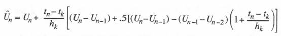
In this case, when the extrapolation interval ![]() , we see from Table 4.2 that the extrapolation error becomes
, we see from Table 4.2 that the extrapolation error becomes ![]() . Thus the error when using quadratic extrapolation is proportional to
. Thus the error when using quadratic extrapolation is proportional to ![]() , compared with
, compared with ![]() for linear extrapolation.
for linear extrapolation.
We now examine the effect of using either the above linear or quadratic extrapolation formulas to compute the input data sequence ![]() from a fixed-step input
from a fixed-step input ![]() , where
, where ![]() is equal to the mean value of the variable step
is equal to the mean value of the variable step ![]() . Again we use our example second-order system simulation with the variable step size
. Again we use our example second-order system simulation with the variable step size ![]() , as shown in Figure 9.1. The resulting errors in simulated output
, as shown in Figure 9.1. The resulting errors in simulated output ![]() , when using variable-step, second-order predictor integration are shown in Figure 9.12, along with the errors when the input data points
, when using variable-step, second-order predictor integration are shown in Figure 9.12, along with the errors when the input data points ![]() are exact, as assumed in all previous examples in this chapter. Clearly the quadratic extrapolation produces better results than linear extrapolation. With the acceleration-limited step input of Eq. (3.176), it should be noted that the quadratic formula produces exact extrapolation results as long as the input acceleration remains constant over the interval from
are exact, as assumed in all previous examples in this chapter. Clearly the quadratic extrapolation produces better results than linear extrapolation. With the acceleration-limited step input of Eq. (3.176), it should be noted that the quadratic formula produces exact extrapolation results as long as the input acceleration remains constant over the interval from ![]() to
to ![]() , since in this case
, since in this case ![]() is itself a quadratic function of time. Thus it is only for the intervals which include a step change in acceleration, i.e., at
is itself a quadratic function of time. Thus it is only for the intervals which include a step change in acceleration, i.e., at ![]() , T and 2T with T = 1.2, that quadratic extrapolation introduces errors in
, T and 2T with T = 1.2, that quadratic extrapolation introduces errors in ![]() .
.
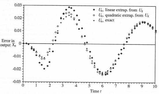
Figure 9.12. Effect of extrapolation in converting fixed-rate data points ![]() to variable-step input data points
to variable-step input data points ![]() , for second-order predictor integration.
, for second-order predictor integration.
We consider next the multi-rate input/output case, where the fixed step ![]() is significantly smaller than the mean of the variable step
is significantly smaller than the mean of the variable step ![]() . Here we use the same example employed in Section 9.4, with
. Here we use the same example employed in Section 9.4, with ![]() and second-order predictor integration as the extrapolation method for producing the multi-rate output. In this case both input and output frame rates are 2.5 times the mean frame rate of the variable-step simulation. Because
and second-order predictor integration as the extrapolation method for producing the multi-rate output. In this case both input and output frame rates are 2.5 times the mean frame rate of the variable-step simulation. Because ![]() has been reduced from 0.2 to 0.08, the extrapolation errors will be much smaller. In fact, when quadratic extrapolation is used to provide the variable-step input data points, the simulation errors can barely be distinguished from those shown earlier in Figure 9.7, where exact input data points
has been reduced from 0.2 to 0.08, the extrapolation errors will be much smaller. In fact, when quadratic extrapolation is used to provide the variable-step input data points, the simulation errors can barely be distinguished from those shown earlier in Figure 9.7, where exact input data points ![]() were assumed. When linear extrapolation is used to compute the variable-step
were assumed. When linear extrapolation is used to compute the variable-step ![]() from the fixed-step
from the fixed-step ![]() , the results in Figure 9.13 are obtained, which now show only a slight error introduced because of the extrapolation.
, the results in Figure 9.13 are obtained, which now show only a slight error introduced because of the extrapolation.
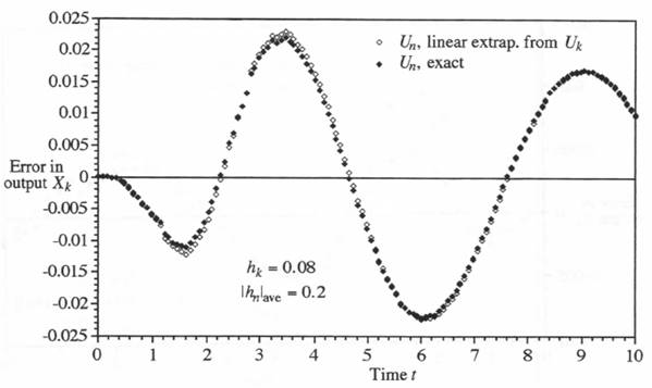
Figure 9.13. Effect of linear extrapolation to convert multi-rate data points ![]() to variable-step input data points
to variable-step input data points ![]() for second-order predictor integration.
for second-order predictor integration.
In Section 9.5 we observed that the use of variable-step third-order predictor integration in our example simulation reduces significantly the simulation output errors obtained when utilizing second-order predictor integration. This is evident in comparing the results shown in Figure 9.8 with those of Figure 9.3. On the other hand, the extrapolation errors resulting from the conversion of fixed-step input data points ![]() to variable-step input data points
to variable-step input data points ![]() , as considered in this section, depend only on the extrapolation method and not the integration algorithm used in the variable-step simulation of the dynamic system. We therefore conclude that the input extrapolation errors will have a greater relative effect on the output errors when using the more accurate, third-order variable-step predictor integration method. This is confirmed in Figure 9.14, which shows the errors in simulated output
, as considered in this section, depend only on the extrapolation method and not the integration algorithm used in the variable-step simulation of the dynamic system. We therefore conclude that the input extrapolation errors will have a greater relative effect on the output errors when using the more accurate, third-order variable-step predictor integration method. This is confirmed in Figure 9.14, which shows the errors in simulated output ![]() when using quadratic extrapolation to convert the fixed-rate real-time input data points
when using quadratic extrapolation to convert the fixed-rate real-time input data points ![]() to the required variable-rate input data points
to the required variable-rate input data points ![]() . Also shown in the figure are the output errors when the input data points
. Also shown in the figure are the output errors when the input data points ![]() , are exact. When the extrapolated data points
, are exact. When the extrapolated data points ![]() instead of the exact data points
instead of the exact data points ![]() are used as inputs, Figure 9.14 shows that the simulation output error is nearly doubled. Of course, the use of linear extrapolation to calculate the variable-step input data points
are used as inputs, Figure 9.14 shows that the simulation output error is nearly doubled. Of course, the use of linear extrapolation to calculate the variable-step input data points ![]() will produce even larger output errors. By contrast, the results in Figure 9.12, where second-order instead, of third-order predictor integration is used for the simulation, show that the increase in error caused by quadratic extrapolation of the input data points is relatively small. It should be noted that higher-order extrapolation formulas, such as cubic extrapolation, will not provide further accuracy improvement. This is because of the nature of the acceleration-limited input for our example simulation, with its discontinuous second derivatives.
will produce even larger output errors. By contrast, the results in Figure 9.12, where second-order instead, of third-order predictor integration is used for the simulation, show that the increase in error caused by quadratic extrapolation of the input data points is relatively small. It should be noted that higher-order extrapolation formulas, such as cubic extrapolation, will not provide further accuracy improvement. This is because of the nature of the acceleration-limited input for our example simulation, with its discontinuous second derivatives.
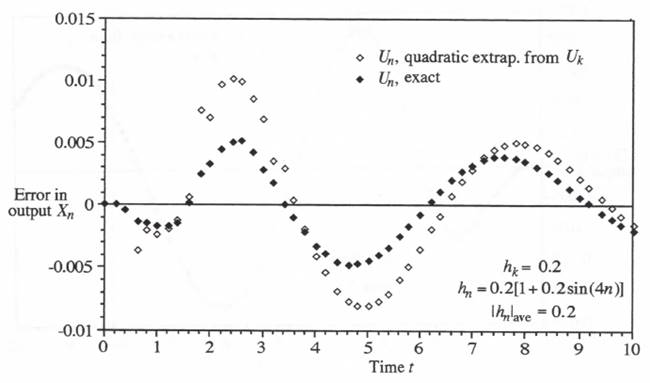
Figure 9.14. Effect of quadratic extrapolation to convert fixed-rate data points ![]() to variable-step input data points
to variable-step input data points ![]() for third-order predictor integration.
for third-order predictor integration.
Finally, we consider the multi-rate input/output case when third-order, variable-step predictor integration is utilized for the simulation. Again we use the same example employed in Section 9.4, with ![]() and third-order predictor integration as the extrapolation method for producing the multi-rate output. Because
and third-order predictor integration as the extrapolation method for producing the multi-rate output. Because ![]() has been reduced from 0.2 to 0.08, the extrapolation errors will be much smaller. As in the case of second-order predictor integration, we find that when quadratic extrapolation is used to provide the variable-step input data points for third-order predictor integration, the simulation errors can barely be distinguished from those shown earlier in Figure 9.9, where exact input data points
has been reduced from 0.2 to 0.08, the extrapolation errors will be much smaller. As in the case of second-order predictor integration, we find that when quadratic extrapolation is used to provide the variable-step input data points for third-order predictor integration, the simulation errors can barely be distinguished from those shown earlier in Figure 9.9, where exact input data points ![]() were assumed. When linear extrapolation is used to compute the variable-step
were assumed. When linear extrapolation is used to compute the variable-step ![]() from the fixed-step
from the fixed-step ![]() , the results in Figure 9.15 are obtained. Comparison with Figure 9.13 shows that here, where third-order predictor integration is used for the simulation, the relative effect of linear extrapolation to produce the variable-step input data points is more noticeable.
, the results in Figure 9.15 are obtained. Comparison with Figure 9.13 shows that here, where third-order predictor integration is used for the simulation, the relative effect of linear extrapolation to produce the variable-step input data points is more noticeable.
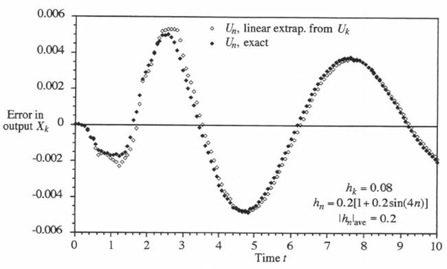
Figure 9.16. Effect of linear extrapolation to convert fixed-rate data points ![]() to variable-step input data points
to variable-step input data points ![]() for third-order predictor integration.
for third-order predictor integration.
From the simulation results in this section it seems clear that variable-step simulation using predictor-integration methods will be improved significantly if multi-rate sampling is employed to generate fixed-rate, real-time inputs to the simulation. This is because the extrapolation formulas used to convert the fixed-rate input data points ![]() to the required variable-rate input estimates
to the required variable-rate input estimates ![]() will be much more accurate for input step sizes
will be much more accurate for input step sizes ![]() which are small compared with the mean of the variable step
which are small compared with the mean of the variable step ![]() used in the simulation.
used in the simulation.
It should be noted that the extrapolation intervals required to produce input data points ![]() for a variable-step real-time simulation from real-time input data points
for a variable-step real-time simulation from real-time input data points ![]() can be reduced substantially if the input data points
can be reduced substantially if the input data points ![]() are not needed at the start of the nth integration frame. This suggests that all computations which do not require
are not needed at the start of the nth integration frame. This suggests that all computations which do not require ![]() should be scheduled first in arranging the order of integration-step calculations. Then, when
should be scheduled first in arranging the order of integration-step calculations. Then, when ![]() is finally needed, enough time may have elapsed that the next data point,
is finally needed, enough time may have elapsed that the next data point, ![]() , may now be available for use in the extrapolation formula, thus reducing the required extrapolation interval.
, may now be available for use in the extrapolation formula, thus reducing the required extrapolation interval.