Chapter 8 – Multi-rate Integration

8.1 Introduction

Multi-rate integration provides a method for improving performance in simulating dynamic systems consisting of identifiable slow and fast subsystems. In multi-rate integration, the fast subsystem is simulated with an integration step size given by  , where   is the slow subsystem step size and N is normally an integer. Thus the integration frame rate   used for the fast subsystem is N times the integration frame rate   used for the slow sub-system, as illustrated in Figure 8.1. In Section 4.9 we analyzed the dynamic errors inherent in generating the fast data-sequence input to the fast subsystem from the slow data-sequence output of the slow subsystem using extrapolation or interpolation formulas. From Figure 8.1 it is also clear that we must generate a slow input data-sequence to the slow subsystem from the fast data-sequence output of the fast subsystem.

 

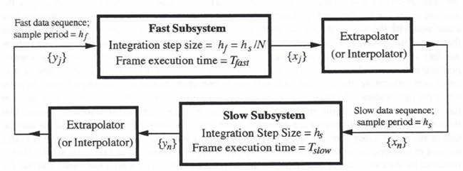
Figure 8.1. Multi-rate integration in simulating combined fast and slow subsystems.

 

If the computer used in the simulation requires   seconds to execute each fast-subsystem integration step and   seconds to execute each slow-subsystem integration step, then the time required to execute N fast subsystem integration steps and one slow subsystem integration step is given by  . Furthermore, if the computer is always utilized with maximum efficiency in a real-time simulation (i.e., no processor idle times), it follows that the mathematical step sizes   and  ,  for fast and slow subsystem integrations are given, respectively, by

 

(8.1)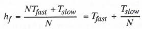     

(8.2)     

From Eqs. (8.1) and (8.2) we see that increasing the multi-rate frame ratio N decreases the step size   for the fast subsystem simulation and increases the step size   for the slow subsystem simulation. In particular, when the time required to execute each fast subsystem integration step is very small compared with the time required to execute each slow subsystem integration step, i.e., when  , it is apparent from Eq. (8.1) that the step size   for the fast subsystem simulation can be reduced quite substantially by making N large. This in turn will improve the accuracy and stability of the fast subsystem simulation. Of course, this is accomplished at the expense of a substantial increase in the step size  , and hence reduced accuracy for the slow subsystem simulation. Thus the choice of N involves a tradeoff, with the optimal N dependent on each particular simulation.*  When  , Eqs. (8.1) and (8.2) show that little or nothing is gained by utilizing multi-rate integration, i.e., by making N > 1.

 

8.2 Scheduling Algorithms

When a single processor is used for multi-rate simulation, it is necessary to determine the order in which the equations for each subsystem are processed. One algorithm that is both simple and logical is one which selects the subsystem with the earliest next-frame time. To illustrate, at the completion of a given integration frame (for either fast or slow subsystem) let   , and   be the discrete times for the fast and slow subsystem frames, respectively, where   is the discrete time associated with the start of the jth fast subsystem frame and   is the discrete time associated with the start of the nth slow-subsystem frame. Then   will be the discrete time corresponding to the j + 1 fast-subsystem frame and   will be the discrete time corresponding to the n + 1 slow-subsystem frame. If  , then the fast subsystem frame is executed next; otherwise, the slow subsystem frame is executed. In this way no single frame, be it for either the fast or slow subsystem, has a completion time that is greater than the completion time for the next frame of the opposite subsystem. Put another way, this scheduling algorithm ensures that the simulation of one subsystem can never fall more than one integration frame behind the simulation of the other subsystem. When applied to the multi-rate example shown in Figure 8.1, this method of scheduling starts the simulation by executing N frames of the fast subsystem. This is followed by the execution of one frame of the slow subsystem, after which the state variables for both fast and slow sub-systems once again represent the same discrete time.

 

A second candidate scheduling algorithm is one which selects the subsystem with the earliest discrete time associated with its current state. Based on the notation introduced above, this algorithm executes a fast subsystem integration step whenever  ; otherwise a slow subsystem integration step is executed. When applied to the multi-rate example shown in Figure 8.1, this method of scheduling starts the simulation by executing one frame of the slow subsystem. This is followed by the execution of N frames of the fast subsystem, after which the state variables for both fast and slow subsystems once more represent the same discrete time.

 

Yet a third scheduling algorithm is based on selecting for execution the integration frame of the subsystem whose next half-frame occurs the earliest. Thus we determine   and   at the beginning of each new integration frame. If  , we execute the fast subsystem integration step; otherwise, we execute the slow subsystem integration step. When applied to the multi-rate example shown in Figure 8.1, this method of scheduling

* See, for example, Haraldsdottir, A., and R.M. Howe, “Multiple Frame Rate Integration,” Proc. of the AIAA Flight Simulation Technologies Conference, Atlanta, Sept. 7-9, 1988, pp 26-35.

starts the simulation by executing N/2 frames of the fast subsystem (assuming N is even). This is followed by the execution of one frame of the slow subsystem. Then the remaining N/2 frames of the fast subsystem are executed, after which the state variables for both fast and slow subsystems once more represent the same discrete time. This scheduling algorithm, which Howe and Lin have described as the method of staggered integration steps,* ensures that the simulation of any one subsystem can never fall more than one-half integration frame behind the other subsystem simulation.

 

The extension of the above scheduling algorithms to multi-rate simulation of more than two subsystems is obvious. Also, the methodology can be applied to non-real-time as well as real-time simulation. To obtain a more complete understanding of the various multi-rate scheduling algorithms, we now consider a specific example.

 

8.3 Example Multi-rate Simulation

Figure 8.2 shows the dynamic system that will be used in this chapter to illustrate multi-rate integration. It represents an aircraft pitch control system consisting of an airframe, autopilot and control-surface actuator. The flight control system output is the aircraft pitch angle  , and the input is the command pitch angle,  . Proportional and rate feedback are used along with   as autopilot inputs. For simplicity we model the airframe dynamics with the following transfer function:

 

 

 

(8.3)

 

Eq. (8.1) represents the short-period dynamics of the linearized longitudinal airframe equations of motion. If we were to include a full nonlinear model for the airframe dynamics, it would not change significantly the multi-rate integration results presented here. The dynamic behavior of the airframe is dominated by the undamped natural frequency,  , of the short-period pitching motion. Here we will assume that  = rad/sec, which is representative of an agile, high-performance aircraft. The airframe will be considered a slow subsystem, and will be simulated with a nominal integration step size of    seconds. In the example simulation we let  ,  , and  . The state equations for the airframe simulation are the following:

(8.4)     

(8.5)     

(8.6)     

(8.7)     

* Lin, K.C., and R.M. Howe, “Simulation Using Staggered Integration Steps. Part II: Implementation on Dual-speed Systems,” Transactions of the Society for Computer Simulation, Vol. 10, No. 4, Dec., 1993, pp. 239-262.

 

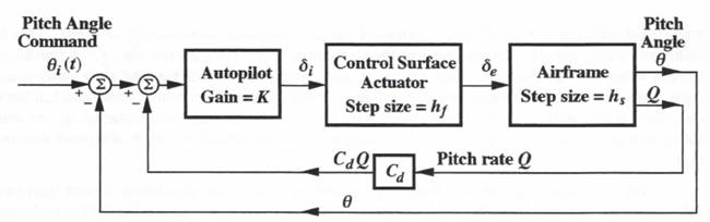
Figure 8.2. Example flight control system.

 

The control surface actuator is modeled as a fourth-order system with the following transfer function:

(8.8)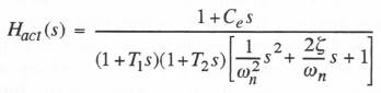     

 

This fourth-order actuator model is based on the closed-loop servo shown in Figure 8.3, i.e., a pure inertia plant driven by a proportional-plus-rate controller with a double lag. In this configuration the state equations are the following:

(8.9)     

(8.10)   

(8.11)   

(8.12)   

 

The following open-loop actuator parameter values are used in the example simulation:  . These lead directly to the following closed-loop parameters for the actuator model represented in the transfer function of Eq. (8.8):   and   The actuator will be considered a fast subsystem to be simulated with a nominal integration step size   seconds. The remaining flight-control system parameters in Figure 8.2 are given by   and  .

 

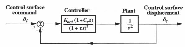
Figure 8.3. Control surface servo actuator.

 

When we simulate the flight control system with the above parameters using a single fixed step size for numerical integration of both the airframe and actuator state equations, then the maximum allowable step size will be governed by the eigenvalue of largest magnitude for the overall closed-loop system. For the case considered here, it turns out that this eigenvalue will be approximately equal to the open-loop eigenvalue of largest magnitude, namely,  . If we use second-order Adams-Bashforth (AB-2) integration with step size h for the simulation, then the AB-2 stability boundary of Figure 3.2 shows that   must be less than 1 for the simulation to remain stable. For   it follows that h < 0.006688, which is an excessively small step size for the airframe simulation. If we employ RK-4 integration, then Figure 3.5 shows that   must be less than 2.8 for a stable simulation, and it follows that h < 0.0187. Again, this is an excessively small step size for the airframe simulation when using RK-4. This is why we turn to multi-rate simulation, where we use a step size   for the actuator simulation that is sufficiently small to ensure an accurate and stable actuator solution, and a larger step size h, for simulating the slower dynamics of the airframe.

 

In the example considered here we will use the AB-2 integration method. As noted above, we let the nominal step sizes for the actuator and airframe simulations be given by   and  , respectively. It follows that the frame ratio   for these step sizes. To obtain a reference solution against which subsequent solutions can be compared to calculate simulation errors, we first run the simulation with  . Figure 8.4 shows the resulting response for an acceleration-limited step input, as defined earlier in Eq. (3.176). We recall that use of the acceleration-limited step input avoids the large errors inherent in predictor integration methods when subjected to discontinuous inputs. Also, the acceleration-limited step is more representative of a physical input that can actually occur. With the input acceleration reversal time of 0.2 seconds used here, the flight-control system response is very close to the response for an ideal unit-step input.

 

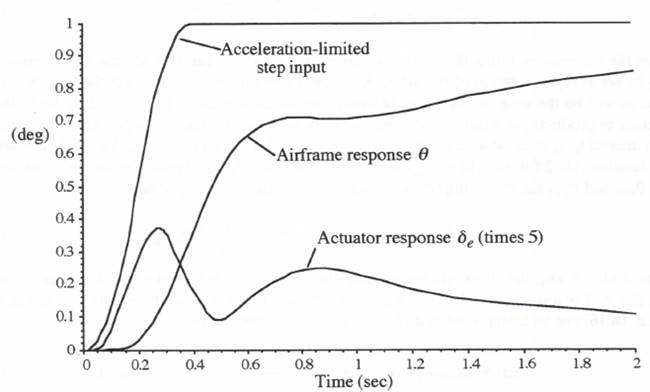
Figure 8.4. Flight control system response to an acceleration-limited step input

 

8.4 Extrapolation Formulas for Interfacing Subsystem Data Sequences

When we perform the simulation using the nominal integration step sizes of 0.002 and 0.02 seconds for the fast and slow subsystems, respectively, it is necessary to use extrapolation to obtain the inputs   and Q to the autopilot every 0.002 seconds from the airframe simulation outputs that occur every 0.02 seconds. In the case of  ,  we first consider linear extrapolation based on   and  , the current and immediate past outputs of the airframe simulation, which correspond to the times  , and  , respectively. Then the formula for  , the value of   at time   based on linear extrapolation, is given by

(8.13)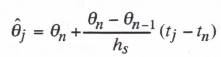   

 

Here  , the integration step size used for the airframe (slow subsystem) simulation. The formula in Eq. (8.13) can be viewed as a representation for   based on the zeroth and first order terms of a Taylor series expansion, where   is a backward difference approximation for the time derivative,  . Since   is available directly as an output of the airframe simulation  , an alternative first-order extrapolation formula for of   is given by

(8.14)   

Table 4.2 in Chapter 4 shows that Eq. (8.14) in general provides a more accurate result than Eq. (8.13) and should be used for first-order extrapolation whenever the time derivative   is available in the simulation.

 

An even more accurate extrapolation formula when   is available is based on second-order predictor integration of   to obtain  . In this case the extrapolation formula becomes

(8.15)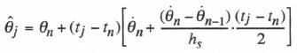   

 

Here the formula includes the second-order term as well as zeroth and first-order terms in the Taylor series representation of  . When AB-2 predictor integration is used in the airframe simulation, as will be the case in our example multi-rate simulation here, Eq. (8.15) has the further advantage of producing a result which agrees exactly with the simulation output when the extrapolation interval  , is equal to the integration step size. Thus when  , Eq. (8.15) reduces to the familiar AB-2 formula  . From Taylor series expansions for   and   the following formula for the extrapolation error is obtained:

(8.16)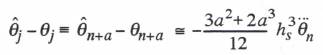   

 

Here  , the dimensionless extrapolation interval, which we introduced previously in Chapter 4. For a sinusoidal data sequence of frequency   and the error in Eq. (8.16) can be interpreted as an extrapolator phase error, which is then given by

(8.17)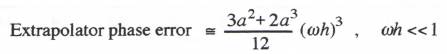   

 

Here the phase error predominates, since the gain error is proportional to  , which is also true for the other three quadratic extrapolation formulas listed earlier in Table 4.2. In addition to providing better accuracy than the linear extrapolation formulas of Eqs. (8.13) and (8.14), we have already noted that the quadratic extrapolation formula of Eq. (8.15) has the added advantage of giving the same result as AB-2 integration when the extrapolation interval is equal to one frame (equivalent to a = 1). This in turn minimizes any transients that might otherwise be caused by the application of the extrapolation formulas in multi-rate simulation when using AB-2 integration.

 

In the case of the pitch rate Q, the time derivative   is not available at the beginning of the nth frame. For linear extrapolation to the fast data sequence values  , we can use the counterpart of the backward difference formula in Eq. (8.13). For quadratic extrapolation the formula based on  ,   and   has already been derived in Section 4.4 and here is given by

(8.18)   

 

The error associated with this extrapolation formula, which is listed in Table 4.2, is larger than the error associated with the predictor integration formula of Eq. (8.15).

 

Next we consider the interface between the fast actuator and slow airframe subsystems in Figure 1. When the two subsystems are simulated using the multi-rate integration step sizes of 0.002 and 0.02 seconds, respectively, no extrapolation is needed to produce the airframe input  . This is because the frame ratio   and therefore every tenth output   from the actuator simulation will exactly represent an airframe input  .

 

8.5 Multi-rate Simulation Results Using Earliest Next-frame Scheduling

In this section we consider multi-rate simulation of the example flight control system when the execution of the fast and slow subsystem integration steps is based on the earliest next-frame time. This was the first scheduling method introduced in Section 8.2. For multi-rate integration step sizes given by   and  , the errors in simulated airframe output   and actuator output   when utilizing AB-2 integration are shown in Figure 8.5. For these results we used Eqs. (8.15) and (8.18), respectively, to compute the fast data sequence points   and   from the slow data-sequence points   and  , although it turns out that the more simple linear extrapolation formulas of Eqs. (8.13) and (8.14) give results that are almost as good for this particular case. As noted above, no extrapolation is required to generate the input data points   for the slow airframe simulation from the output values   of the fast actuator simulation, since here the frame ratio N is an integer and every tenth   corresponds exactly to a   data point. To avoid clutter in Figure 8.5, we have only shown every 10th point in the   data.

 

It is useful to consider a more accurate alternative to AB-2 integration of the airframe input data points   from the actuator simulation. For example, trapezoidal integration based on   and   can be used, with the remaining terms in the state equations integrated with the AB-2 algorithm. Figure 8.6 shows the resulting errors in airframe output compared with the earlier errors when AB-2 integration is used everywhere. The figure demonstrates that a significant improvement in accuracy is obtained simply by replacing AB-2 with trapezoidal when integrating the   input term in the airframe state equations. Although trapezoidal integration represents an implicit

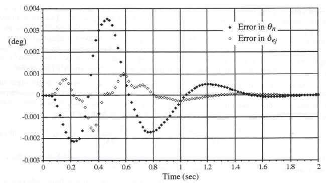
 Figure 8.5. Simulation errors for   using AB-2 integration.

 

method when the state-variable derivatives are functions of the states, it can be used here as an explicit method when applied to the actuator outputs   and  , as obtained by extrapolation from the actuator multi-rate output data points  . Figure 8.7 shows that replacing AB-2 integration with trapezoidal integration of the airframe input   results in an even greater improvement in the accuracy of the simulated actuator output. As before, we only show every 10th data point error in   to prevent cluttering the results displayed in the figure.

 

The accuracy improvement apparent in Figures 8.6 and 8.7 is not surprising when we consider that trapezoidal integration is in general about 5 times more accurate than AB-2 integration. This is evident when we examine the integrator error coefficients   listed in Table 3.1 of Section 3.12. Indeed, there are other more accurate alternatives to AB-2 integration of the   input term in the airframe, state equations. For example, through extrapolation based on the   data points we can obtain  , an estimate of the airframe input half-way through the nth frame. This can then be integrated through simple multiplication by the step size  , which is equivalent to the modified Euler method discussed in Chapter 7. Yet another possibility is to calculate an estimate of the mean value,   of the actuator output over the nth airframe step based on all the multi-rate actuator output data points   which span the nth step. This mean value,  , is then multiplied by the step size   to obtain the contribution of the actuator output   to the overall integration of the first airframe state equation. Indeed, as the frame ratio N becomes very large, a numerical integration based on multiplying the mean value of an input over one integration step by the step size itself approaches the exact integral of the input. When either of these two alternative schemes for integrating   are used in our example simulation here, i.e., integration based on   or integration based on  , results comparable to those shown in Figures 8.6 and 8.7 for the trapezoidal case are obtained.

 

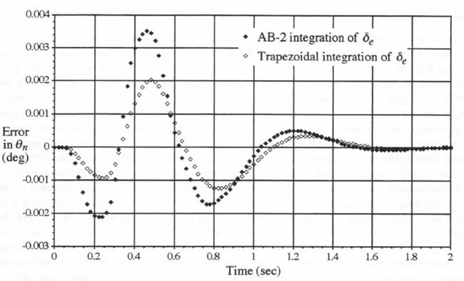
Figure 8.6. Comparison of airframe output errors when the trapezoidal method instead of AB-2 is used to integrate the airframe input .

 

 

Figure 8.7. Comparison of actuator output errors when the trapezoidal method instead of AB-2 is used to integrate the airframe input .

 

8.6 Use of Extrapolation to Produce Multi-rate Simulation Outputs

Thus far in this chapter we have considered multi-rate simulation of a dynamic system with fast and slow subsystems. As noted in Section 8.1, the overall simulation can be run in real time by utilizing Eqs. (8.1) and (8.2) to set the sizes   and   of the fast and slow subsystem integration frames, based on the respective frame execution times   and   together with the frame ratio N. Until now, however, we have not taken into account any specific real-time input and output requirements. As we will see later in this chapter, the real-time input/output requirements in a real-time simulation can play an important role in the selection of multi-rate frame-execution algorithms, as well as the errors introduced by the extrapolation methods needed to utilize real-time inputs and produce real-time outputs. Regardless of whether the overall simulation is to be run in real time or non-real time, there may be instances when it is desirable to provide output data sequences from a simulation at a sample rate that differs from the frame rate used in the numerical simulation. For example, in real-time simulation the dynamic accuracy associated with the output of D to A (Digital to Analog) converters can be improved significantly by driving the converters at an update rate which is a multiple of the real-time integration frame rate, as we have seen in Chapter 4. Also, in both real-time and non-real-time simulation it may be preferable to log data at sample rates that differ from the basic integration frame rates used in the various subsystem simulations. Generation of these multi-rate outputs can be realized using the extrapolation methodology introduced here for multi-rate simulation.

 

As a specific example, we consider again the multi-rate simulation of the flight control system using AB-2 integration, with the actuator and airframe integration step sizes given by   and  , respectively. For both airframe output   and actuator output  , let us further assume that we wish to provide accurate output data with a sample period  . Note that this value of    is non-commensurate with either the 0.002 or 0.02 integration steps used in the simulation to integrate the actuator and airframe state equations, respectively. We employ the predictor-integration extrapolation formula represented by Eq. (8.15) to generate the simulation outputs with step size  . In Figures 8.8 and 8.9 the resulting output errors in   and   are compared with the errors when   and therefore no extrapolation is needed for output data-sequence generation. In both figures the output errors for   fall almost on top of the output errors for  . It should be born in mind that any slight differences between the   and   cases in Figures 8.8 and 8.9 represent deviations in the output errors, where the errors themselves are quite small to begin with. As noted earlier, the second-order predictor-integrator formula of Eq. (8.15) is a particularly effective extrapolation algorithm, since it reduces to the AB-2 algorithm when the extrapolation interval is equal to the integration step size. This in turn minimizes any discontinuities that would normally occur when using other extrapolation methods, regardless of their order.

 

8.7 Alternative Multi-rate Scheduling Algorithms

In Section 8.2 we presented three algorithms for scheduling the order in which the individual subsystem frame calculations are executed in multi-rate integration. Until now we have used only the first of these scheduling algorithms for multi-rate simulation of the example flight control system of Figure 8.2, namely the one based on executing the subsystem with the earliest occurrence of the next full-frame time. To obtain a more detailed understanding of this multi-rate scheduling algorithm, we turn to the timing diagram shown in Figure 8.10. The diagram is based

 

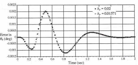
Figure 8.8. Comparison of airframe output errors for output step size   airframe integration step  actuator integration step 

 

 

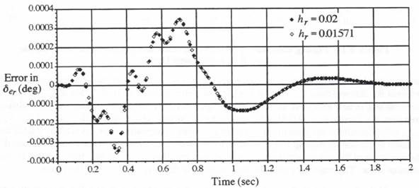
Figure 8.9. Comparison of actuator output errors for output step size  airframe integration step  actuator integration step 

 

on the example multi-rate simulation of the flight control system, with the integration step size for the fast control-surface actuator subsystem given by   and the step size for the slow airframe subsystem given by  . Simulation time is shown along the horizontal axis and computer execution time along the vertical axis in the diagram. Also, the execution of actuator integration steps is indicated by the short line segments and the execution of airframe integration steps by the long line segments. The diagram shows that the simulation starts with the execution of 10 actuator integration steps, corresponding to    After the 10^th

 

 

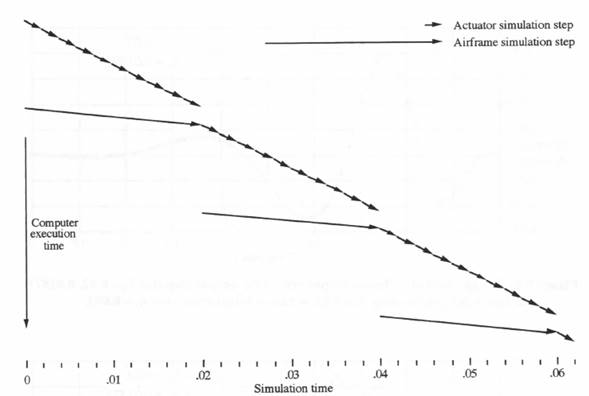
Figure 8.10. Timing diagram for multi-rate scheduling algorithm based on the earliest next-frame time.

 

actuator step has been completed, the discrete time   for the next airframe step is equal to 0.02, whereas the discrete time   for the next actuator step is equal to 0.022. Since   the airframe step is now executed, as indicated in Figure 8.10. After this execution, the next airframe step time has increased to 0.040, whereas the next actuator step time is still 0.022. Thus   which results in the execution of the next actuator integration step, as well as 9 additional actuator steps, corresponding to   This is then followed by the execution of the second airframe integration step, resulting in   followed by 10 more actuator steps. The multi-rate sequencing continues in this way, as shown in the figure.

 

At the beginning of the execution of each airframe integration step, the diagram in Figure 8.10 shows that the 10 actuator steps spanning the next airframe step have already been computed. This gives us the option of utilizing the average value,   of the actuator output over the nth airframe step for a modified-Euler integration of  . Alternatively, we can use trapezoidal integration based on   and   or AB-2 integration based on   and    Earlier we noted that either trapezoidal integration or modified Euler integration based on averaging produces more accurate results than AB-2 integration of the actuator input   to the airframe simulation.

 

Figure 8.10 also shows that the extrapolated values   of the airframe output, as needed for inputs to the multi-rate actuator simulation, require extrapolation intervals   which can range in size up to one whole airframe step,    By using the extrapolation formula of Eq. (8.15) which is based on the AB-2 predictor integration algorithm, we were able to minimize both extrapolation errors and discontinuities caused by those errors in the calculation of   despite the large extrapolation interval. On the other hand, in the calculation of the extrapolated airframe pitch-rate output    where   is not available, we were forced to use the quadratic formula of Eq. (8.18), which can cause a significant discontinuity at the maximum extrapolation interval.

 

The problem of extrapolating the airframe outputs   and Q over one airframe step   can be eliminated if we use the multi-rate scheduling algorithm based on selecting for execution the subsystem with the earliest current-frame time. This results in the timing diagram shown in Figure 8.11. In this case the airframe integration step is executed first, followed by the 10 actuator steps. Now the values   of the airframe output, as needed for inputs to the multi-rate actuator simulation, can be obtained by extrapolation, with the extrapolation interval   ranging between   and 0. The formulas in Table 4.2 show that the extrapolation errors are much less in this case, which actually corresponds to interpolation over the interval from   to    Also, there is no longer a problem with extrapolation discontinuities. This is because the extrapolation errors vanish at both   and    However, the price we have paid for using this scheduling algorithm is the loss of availability of the 10 actuator outputs   spanning each new airframe step, since in this case the airframe step is computed first. It follows that only predictor integration of   can be considered, and we have already seen that AB-2 integration of be produces less accurate results.

 

 

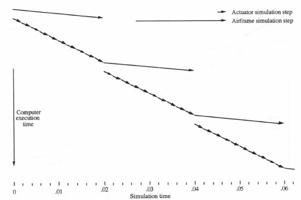
Figure 8.11. Timing diagram for multi-rate scheduling algorithm based on the earliest current-frame time.

 

The third scheduling algorithm introduced in Section 8.2 is based on selecting for execution the integration frame of the subsystem whose next half-frame occurs the earliest. This third method represents a compromise algorithm which retains the advantages and reduces the disadvantages of the first two scheduling algorithms. Thus we determine   and   at the beginning of each new integration frame. If   we execute the actuator integration step; otherwise, we execute the airframe integration step. This alternative scheduling algorithm ensures that the simulation of any one subsystem can never fall more than one-half integration frame behind the other subsystem simulations. Figure 8.12 shows the timing diagram of the individual actuator and airframe integration steps that occur when using this scheduling method. The diagram shows that the simulation starts with the execution of 5 actuator integration steps, corresponding to    and 0.010. At this point,   is less than   and the airframe integration step is executed, after which    This is followed by the execution of 10 actuator integration steps, corresponding to   since for each step   For the following step, however,   is less than   and the airframe step is executed. In this fashion the multi-rate integration proceeds as shown in Figure 8.12, with 10 actuator steps per airframe step. Note that each airframe step is executed when the multi-rate actuator time reaches the point halfway through the airframe step. It follows that the most recently computed actuator output at the start of the nth airframe integration step represents the actuator output   half-way through

 

 

 

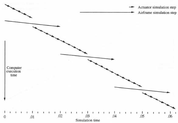
Figure 8.12. Timing diagram for multi-rate scheduling algorithm based on the earliest next half-frame time.

 

the airframe step. This can then be used to provide the input for modified Euler integration of   in the first airframe state equation, which will result in a sizeable improvement in overall simulation accuracy.

 

When each sequence of 10 actuator integration steps is initiated, it is also apparent from Figure 8.12 that the airframe output half-way through the 10-step actuator sequence has already been calculated. It follows that the extrapolation intervals needed to compute the multi-rate actuator inputs   and   range from   to   (i.e., -0.01 to +0.01).  When the original multi-rate scheduling algorithm illustrated in Figure 8.10 is used, we have seen that the extrapolation interval needed to compute   and   ranges from 0 to    i.e., double the maximum extrapolation interval for the scheme in Figure 8.12. This can cause significantly larger extrapolation errors, especially when using the quadratic formula of Eq. (8.17) or either of the linear extrapolation formulas given by Eqs. (8.12) and (8.13).

 

Thus the multi-rate scheduling algorithm illustrated in Figure 8.12 permits more accurate generation of the multi-rate outputs needed to interface the slow subsystem to the fast subsystem. As noted above, it also provides a convenient calculation of the input half-way through the slow-subsystem frame, as required to interface the fast subsystem to the slow subsystem when using modified Euler integration.

 

When the third multi-rate scheduling algorithm illustrated in Figure 8.12 is used for multi-rate simulation of our example flight-control system, the resulting errors in airframe output   and actuator output   are shown in Figure 8.13. Comparison with the previous results in Figure 8.5 shows that the simulation errors have been reduced substantially by utilizing the next half-frame instead of the next full-frame scheduling algorithm. Both simulations employ the same formulas, as given in Eqs. (8.15) and (8.18), for the extrapolations needed for slow-to-fast subsystem interfacing. Also, both simulations use AB-2 integration, with the exception that the simulation in Figure 8.13 uses modified Euler integration of the actuator output   instead of AB-2 integration based on   and  . This is the primary reason for the better accuracy, although the smaller peak extrapolation intervals associated with the next half-frame scheduling algorithm also contribute to the improved accuracy.

 

On the other hand, if we compare Figure 8.13 with the earlier results in Figures 8.6 and 8.7, where trapezoidal integration of   is employed, we see that the errors in Figure 8.13 are somewhat larger. This is true in spite of the fact that the modified Euler method using   is more accurate (local truncation error proportional to  ) than the trapezoidal method using   and   (local truncation error proportional to  ). This apparent inconsistency is probably explained by the negative coefficient of the trapezoidal truncation error, which results in a partial cancellation of the error associated with the AB-2 integration that follows (truncation error proportional to  ).

 

When the earliest next-half-frame scheduling algorithm utilized for Figure 8.13 is employed, we should again note that the maximum required extrapolation interval in the formulas used to generate the slow-to-fast data-sequence conversions is one-half of an integration step. On the other hand, the earliest next-full-frame scheduling algorithm, which was utilized for the simulations in Section 8.5, requires a maximum extrapolation interval of one full integration step in the formulas used to generate the slow-to-fast data-sequence conversions. This results in significantly larger extrapolation errors when implementing the slow-to-fast data interface calculations. We were able

 

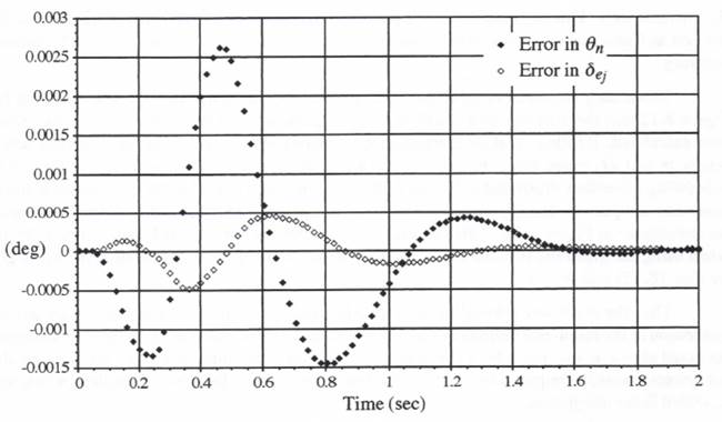
Figure 8.13. Flight-control system simulation errors when using the scheduling algorithm based on the earliest half-frame time;   

 

to minimize the effect of these errors on the overall multi-rate simulation accuracy by employing extrapolation based on the same algorithm used for numerical integration of the state equations, e.g., second-order predictor integration.

 

When the interface variable and its time derivative are not states, however, the predictor-integration extrapolation formula cannot be used, and a different extrapolation algorithm must be employed, e.g., the quadratic formula of Eq. (8.18) to obtain   from  . The resulting discontinuities introduced at the maximum extrapolation interval explain the higher frequency transient evident in the actuator simulation errors of Figures 8.5 and 8.7. When the multi-rate scheduling algorithm based on the earliest next-half frame is used, Figure 8.13 shows that these higher frequencies are no longer present in the actuator error transient. This is because the factor of two decrease in the maximum extrapolation interval reduces, in turn, the quadratic extrapolation error by a factor of more than three (a = 0.5 instead of a = 1), according to Eq. (4.26), with a corresponding reduction in   discontinuity.

 

On the other hand, the scheduling algorithm based on the next full-frame occurrence permits the use of fast data-sequence averaging over one full slow frame. This average can then be integrated in the first slow-subsystem state equation using the modified-Euler method. This in turn can improve substantially the multi-rate simulation accuracy, as opposed to the AB-2 method used for the remaining integrations. Also, integration based on the average input can eliminate the deleterious effects of aliasing when the slow frame-rate frequency is less than twice the highest frequency contained in the fast subsystem output. When scheduling based on the earliest next half-frame occurrence is used, the fast data-sequence values are only available over the first half of the slow subsystem frame, which precludes the use of averaging over the whole frame.

 

It is therefore apparent that neither scheduling algorithm is superior in all cases. If optimal multi-rate integration scheduling is to be achieved for any given simulation, it will be necessary to try both schemes to determine which is the most effective. However, as noted in Section 8.6, we have yet to consider the implications of real-time input and output requirements in real-time simulation. These requirements can be very important in the choice of a multi-rate scheduling method, as we shall see in the next section.

 

8.8 Multi-rate Integration with Real-time Inputs and Outputs

When a single processor is used for real-time multi-rate simulation and real-time inputs and/or outputs are required, special care must be taken in scheduling the various multi-rate integration-step calculations in order to minimize errors caused by latencies in generating the data for real-time inputs and outputs. Again, we utilize the example flight control system of Figure 8.2 for illustrative purposes. Since we will now be concerned exclusively with real-time simulation, it is important to consider the times required to execute the fast actuator and slow airframe integration steps. As a specific example, we assume here that these execution times are given by   and   second. Instead of the frame-ratio N = 10 used up to now for our multi-rate simulations, we will let the frame ratio N = 8. Then, according to Eqs. (8.1) and (8.2), for maximum real-time computational efficiency the mathematical step size for the actuator simulation is given by   and the mathematical step size for the airframe simulation is given by   The total processor execution time for 1 airframe step and the accompanying 8 actuator steps is then equal to 0.01 +8(0.001) = 0.018 sec. Since this is the same as the mathematical size   used for each airframe simulation step, as well as the mathematical size   used for each 8 actuator simulation steps, it follows that the simulation runs exactly at real-time speed.

 

As a first example of multi-rate scheduling, let us use the algorithm based on executing the subsystem integration step with the earliest next half-frame time, which was illustrated earlier in the timing diagram of Figure 8.12. Furthermore, let us assume that the pitch-angle input command   is a real-time input, and that real-time output data sequences from both the actuator and airframe simulations are required. Here again, to better understand the scheduling of individual actuator and airframe integration-step calculations, as well as the timing problems associated with utilizing real-time inputs and producing real-time outputs, it is useful to construct a timing diagram. This has been done in Figure 8.14 for the overall real-time multi-rate simulation. In this diagram, the horizontal axis represents real time (positive to the right) and the vertical axis represents mathematical simulation time (positive downward). Note that the axes here are just the reverse of those used earlier in Figure 8.12. The diagram in Figure 8.14 has been constructed using the specific example step sizes and step execution times given above, namely,   and   for the actuator simulation, and   and   for the airframe simulation. Events which occur in real time, such as real-time input samples   all lie on a straight line through the origin with slope of -1. Events which occur ahead of real time lie below this straight line, and events that occur behind real time lie above this straight line.

 

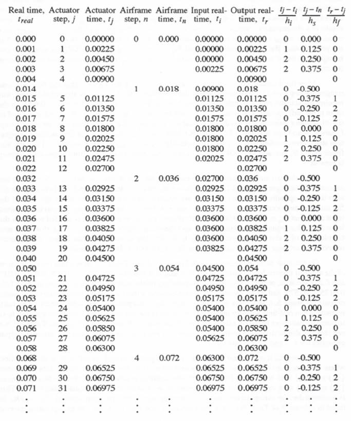
In Figure 8.14 it is apparent that 4 actuator integration steps are scheduled initially (j = 1, 2, 3, 4), followed by a single airframe step (n = 1) and 4 more actuator steps (j = 5, 6, 7, 8). The sequence is then repeated in the same fashion, i.e., 4 actuator steps (j = 9, 10, 11, 12), 1 airframe step (n = 2) and 4 actuator steps (j = 13, 14, 15, 16), for each follow-on major iteration. Both the mathematical simulation time (   or   ) and the corresponding real time (  ) associated with the completion of each actuator or airframe integration step are listed in Table 8.1.

 

Reference to both Figure 8.14 and Table 8.1 shows that the initial 4 actuator steps, which end with   and 0.009, respectively, are completed in real time at   and 0.004 seconds, respectively. Thus the actuator output is calculated ahead of real time in each case, and is therefore available as a real-time output with no latency. On the other hand, at the beginning of the 2nd actuator step, which occurs at   the required real-time input   corresponding to   is not yet available. In this case the required

 

 

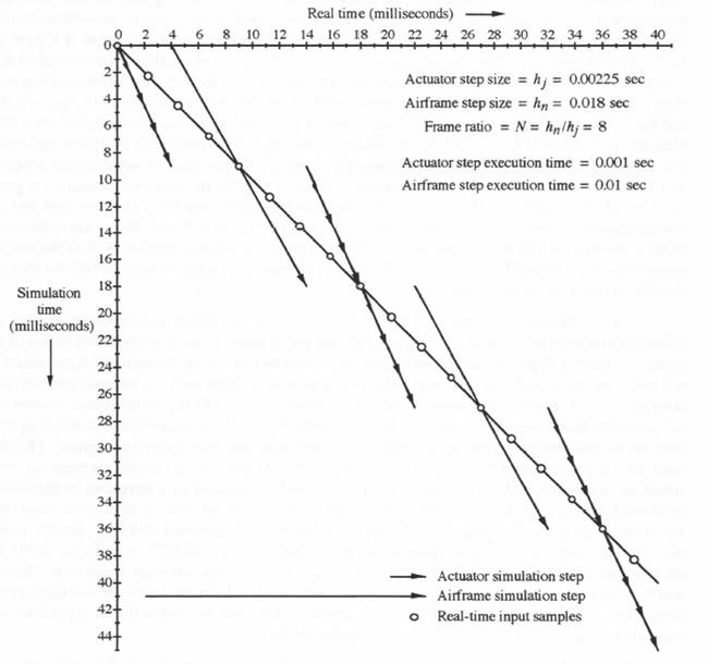
Figure 8.14. Timing diagram for real-time multi-rate simulation with scheduling based on the earliest next half-frame occurrence.

 

Table 8.1

Integration-step Indices, Step Times and Extrapolation Intervals for Multi-rate Integration with Fixed Fast and Slow Integration Steps; Frame-ratio N= 8.

 

 

input   can only be estimated using extrapolation based on  ,  , . The extrapolation interval   for this estimate is equal to 0.00225. This in turn represents a dimensionless extrapolation interval,  , equal to 1, as indicated in row 2, column 8 of Table 8.1. Similarly, at the beginning of the third actuator step, which occurs at  , the required real-time input   corresponding to   is not yet available, nor is the previous input  . Thus the required input   must again be estimated using extrapolation based on  ,  ,  . This now results in a dimensionless extrapolation interval of 2. At the beginning of the fourth actuator step, which occurs at  , the required real-time input    corresponding to   is not yet available. But now the real-time input   corresponding to    is available, and extrapolation based on  ,  ,  , can be used to estimate   with a dimensionless extrapolation interval of 2.

 

After the 4 actuator steps have been executed, Figure 8.14 shows that the first airframe integration step (n = 1) is executed. When the modified Euler integration algorithm is used, this requires the actuator output   half-way through the airframe step, i.e., at  , as the input to the airframe state equations. But this actuator output has just been calculated at the end of the 4th actuator step and hence is directly available as an input for the first airframe integration step. Figure 8.14 and row 6, column 5 in Table 8.1 both show that the end of the first airframe integration step, corresponding to  , actually occurs at   seconds. Thus the airframe output   is available 0.004 seconds ahead of real time and no real-time output-data latency is present.

 

After the first airframe step has been executed, the next 4 actuator steps (j = 5, 6, 7, 8) are executed. Both Figure 8.14 and Table 8.1 show that the calculations for each of these steps begin after the corresponding input data points   are available in real time. For example, the start of the 5th actuator step occurs at   sec, whereas the real time corresponding to the required input data point   is    sec. It follows that no extrapolation is needed to obtain the input data value required for actuator step 5, and the extrapolation interval  ,  shown in row 6, column 8 of Table 1, is therefore equal to 0. For the same reason, the input extrapolation intervals for actuator steps 6, 7 and 8 are also 0, i.e., no extrapolation is needed.

 

On the other hand, reference to both Figure 8.14 and Table 8.1 shows that the calculation of the actuator outputs for actuator steps 5, 6, 7 and 8 is concluded at   = 0.015, 0.016, 0.017 and 0.018 seconds, respectively. The corresponding mathematical simulation times are 0.01125, 0.0135, 0.01575, and 0.018 seconds. It is immediately apparent that the calculations of actuator outputs for steps 5, 6 and 7 are completed after the corresponding real times occur. The only recourse when real-time actuator outputs are required in the simulation with step size equal to   is to compute estimates based on extrapolation. From rows 7, 8 and 9 in column 8 of Table 8.1 we see that the dimensionless extrapolation intervals required for these real-time actuator output estimates are 1, 2 and 2, respectively.

 

In Figure 8.2 it is apparent that the airframe outputs   and Q are fed back to the autopilot, where they become inputs to the actuator simulation. It follows that the output data sequences   and   with step size   from the airframe simulation must be converted to data sequences   and   with step size   in order to serve as inputs to the actuator simulation. This is accomplished by extrapolation, where the dimensionless extrapolation interval,  , is listed in column 9 of Table 8.1. For the example frame ratio of N = 8, the extrapolation interval ranges between   and  , as shown in the table. Note that negative extrapolation intervals actually represent interpolation.

 

In summary, we have seen that multi-rate integration-step execution based on the earliest next half-frame occurrence for the specific example considered here results in the execution of 4 actuator steps, 1 airframe step, and 4 actuator steps. This sequence is then repeated indefinitely in the implementation of the multi-rate simulation with frame-ratio N = 8. Again, based on the step execution times assumed in our example, extrapolation of real-time input samples over intervals as large as 2 actuator steps is required to furnish the inputs for the first 4 actuator steps. Also, extrapolation intervals as large as 2 actuator steps are required to furnish real-time actuator outputs at the actuator frame rate. Finally, extrapolation intervals ranging between 0.375 and -0.5 times the airframe step size   are required to generate the required multi-rate interface data sequence for the fast actuator simulation from the slow airframe simulation.

 

In describing the scheduling of multi-rate integration steps, we have not considered the possibility of breaking each slow airframe step into a number of substeps, ideally N, where the frame ratio N is 8 in our specific example. If the computer code in these substeps can be arranged so that each of the 8 airframe substeps has approximately the same execution time, then the extrapolation intervals needed to accept real-time inputs and provide real-time outputs can clearly be reduced to less than one integration step. On the other hand, subdividing each slow airframe step into N substeps of roughly equal execution time may be a non-trivial task. It may also generate significant associated overhead when implemented in the real-time simulation program. For these reasons this option may prove to be unattractive.

 

Another possibility is to consider alternatives to the algorithm represented in Figure 8.14 and Table 8.1 for scheduling the order of multi-rate integration-step executions. For example, we might first execute the single airframe step, followed by the N actuator steps, which is the second candidate scheme described in Section 8.2. This would immediately eliminate the requirement for extrapolations from real-time input data to obtain the required actuator inputs for each actuator integration step, since the time   associated with every actuator step will always occur later than the corresponding real-time input. On the other hand, if real-time actuator outputs are required, starting the N actuator integration steps only after the entire airframe integration step has been completed may now require extrapolation intervals up to N/2 actuator steps or more. This in turn can result in unacceptable real-time output errors.

 

Clearly there are many ways of scheduling the execution of multi-rate integration steps for single-processor simulations requiring real-time inputs and outputs. As in the non-real-time case, the optimal scheduling method will depend on the specific system being simulated, as well as the real-time input and output requirements. It is believed that the scheduling methodology represented in Figure 8.14 and used in the additional examples in this section represents a reasonable approach for a simple and accurate scheme that is straightforward to implement.

 

We now reexamine the multi-rate simulation of the flight control system of Figure 8.2 with the added requirement of real-time inputs and outputs, as described above. In order to force the actuator response   to exhibit larger high-frequency components, we reduce the step reversal time T from 0.02 to 0.005 seconds. This results in the actuator and airframe reference solutions shown in Figure 8.15, which were obtained with  . Comparison with the earlier solutions in Figure 8.4 shows the expected increase in actuator high-frequency transient.

 

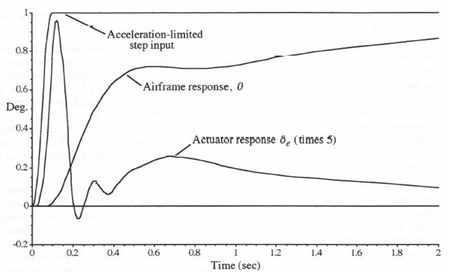
Figure 8.15. Response of flight-control system to an acceleration-limited unit-step input.

 

 

8.9 Simulation with Real-time Inputs and Outputs for the Frame-ratio N = 8

We now consider multi-rate real-time simulation of the flight control system using the next-half-frame scheduling algorithm illustrated in Figure 8.14 and Table 8.1, with actuator and airframe integration step sizes given by   and  , respectively (frame-ratio N = 8). The AB-2 method is used for all integrations except the integration of the actuator input   to the first airframe state equation, which is performed using modified Euler integration based on  . As in the earlier simulation examples in this chapter, the required fast actuator inputs are generated from the slow airframe outputs using the predictor-integration extrapolation formula of Eq. (8.15) for the pitch angle   and the quadratic extrapolation formula of Eq. (8.18) for the pitch rate Q. Extrapolation based on Eq. (8.15) is utilized when required to generate the real-time actuator outputs with sample-period   from the simulation outputs  . In the same way, extrapolation based on Eq. (8.18) is utilized when required to generate the inputs   for the actuator simulation from the real-time input   with sample-period  .

 

The resulting errors in real-time outputs from the actuator and airframe simulation are shown in Figure 8.16. As noted above in Section 8.8, no extrapolation is required to generate the input data points   for the slow airframe simulation from the output values   of the fast actuator simulation, since here the frame ratio N is an even integer and every 8th   corresponds exactly to a   data point (j = 4, 12, 20, … in Table 8.1). Also, no extrapolation is needed to generate the airframe outputs   in real time, since they are actually computed ahead of real time (n = 1, 2, 3, … in Table 8.1). To avoid clutter in Figure 8.16, we have only shown every 8th data point in the real-time actuator outputs. In this case the actuator simulation outputs occur in real time (j = 8, 16, 24, … in Table 8.1)

 

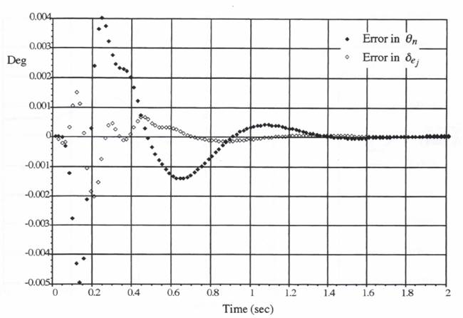
Figure 8.16. Real-time simulation output errors for h_s = 0.018, h_f  = 0.00225 (frame ratio N = 8).

 

and no extrapolation is needed. On the other hand, to generate the real-time actuator output data with sample-period   rather than  ,  extrapolation is required for 3 out of each 8 data points (column 10, rows 7, 8, 9; 16, 17, 18; 25, 26, 27; etc., in Table 8.1). Figure 8.17 shows the real-time actuator output errors for this higher sample rate, where only the first 0.6 seconds of the solution is plotted, again for better display of the individual data points. Despite the fact that the real-time actuator outputs must be computed from the simulation outputs using extrapolation intervals as large as 2 integration steps, the figure demonstrates that the resulting scatter in the data points is almost negligible. Here again it should be noted that we are looking directly at the errors in real-time actuator output in Figure 8.16, where to begin with the errors themselves are quite small.

 

8.10 Simulation Results for Frame-ratios N = 2, 4, 6, 8 and 10

For the simulation above in Section 8.9, we selected N = 8 as the multi-rate frame ratio. For an actuator step-execution time   second and an airframe step-execution time   second, this resulted in real-time integration step sizes given by   and   for the actuator and airframe simulations, respectively. In this section we consider the multi-rate simulation accuracy for alternative frame ratios while maintaining the previous actuator and airframe step-execution times. In order to continue to avoid the requirement of extrapolation in the

 

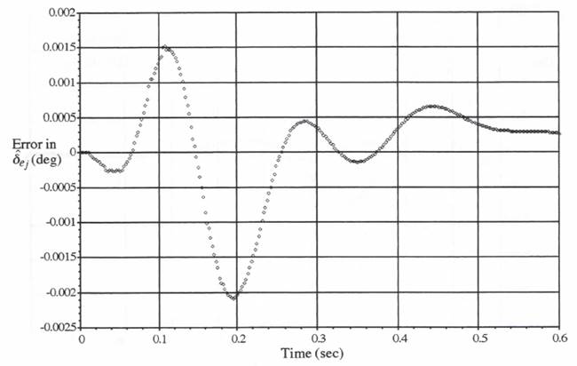
Figure 8.17. Real-time errors in actuator output with sample period = h_f = 0.00225; frame ratio N = 8.

 

actuator-to-airframe data interface, we consider only even-integer frame ratios. The resulting errors in airframe output   are shown in Figure 8.18 for N = 2, 4, 6 and 10, as well as the original frame-ratio N = 8. Note that the errors become less as N is decreased. The reason for this is that the airframe step size   becomes less for smaller values of the frame ratio N, as is evident in Eq. (8.2). For example, for N = 6, the total computer execution time for 6 actuator steps and 1 airframe step is equal to 6(0.001) + 0.01 = 0.016 seconds. For real-time simulation with no computer pauses between the execution of integration steps, this means that the airframe step size is now given by   = 0.016, compared with   = 0.018 when N = 8.  Since the global integration truncation errors are proportional to   when using the second-order AB-2 algorithm, the errors in   for N = 6 will be approximately (0.016/0.018)² or 0.69 times the errors for N = 8. In the same way, Eq. (8.2) shows that   = 0.014 and 0.012 for N = 4 and 2, respectively, whereas for N = 10,   = 0.020. Note also that the spacing   between the data points in Figure 8.18 becomes less as N is decreased and hence   decreases.

 

On the other hand, as the frame-ratio N decreases, the step size   of the actuator simulation increases. Using Eq. (8.1) with   = 0.001 second and   = 0.01 second, we determine that the actuator integration step sizes for N = 10, 8, 6, 4 and 2 are given, respectively, by 0.002, 0.00225, 0.002667, 0.0035, and 0.006. In this case we expect the actuator simulation errors to increase as N decreases. Figure 8.19, which shows the error in computed actuator output for N = 10, 8, 6, and 4, confirms that this is indeed the case. As before, to avoid clutter we show only every Nth actuator-error data point in Figure 8.19. The figure does not include the errors for N = 2,

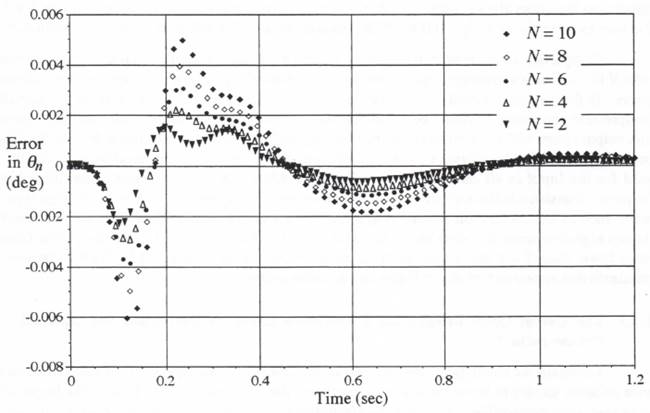
Figure 8.18. Error in real-time airframe output  for different frame-rate ratios N.

 

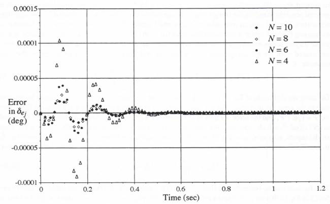
Figure 8.19. Error in real-time actuator output  for different frame-rate ratios N.

 

since the corresponding actuator step size of   = 0.006 results in errors that are several times larger than the errors already shown for N = 4. This is because the 0.006 actuator step size for N = 2 is very close to the value   = 0.006689 that causes an unstable solution, as noted in Section 8.3.

 

Comparison of the results in Figures 8.18 and 8.19 shows that the choice of optimal frame-ratio N for real-time simulation depends on the relative weight given airframe errors versus actuator errors. In this regard it would appear that our original selection of N = 8 represents a reasonable compromise. However, it should be noted that the relative size of airframe versus actuator simulation output errors will, for a given frame-ratio N, depend very much on the input   to the flight control system. The acceleration-limited step input with acceleration-reversal time T = 0.05, as used for the input in all our examples in Sections 8.9 and 8.10, does excite significant high-frequency transients in the actuator output, as can be seen in Figure 8.15. A more benign type of input, such as an acceleration-limited step with T much larger than 0.05, will result in a smaller startup high-frequency transient in the actuator output. This in turn will favor the use of frame-ratios lower than N = 8, since now the simulation errors will be dominated by the low-frequency transients that appear in both the airframe and actuator outputs.

 

8.11 The Use of Local Integration Truncation Error to Determine the Optimal Frame-ratio N

To obtain the simulation errors shown in Figures 8.16 through 8.19, we subtracted a reference solution known to be extremely accurate from the solutions obtained using the larger step sizes that were compatible with real-time simulation. In general, a reference solution can be computed to any desired accuracy by using a sufficiently small integration step size along with higher-order integration methods, although this may require the use double-precision calculations to prevent excessive round-off errors. However, in a hardware-in-the-loop simulation, it is not in general possible to reduce the integration step size below the value already utilized for the real-time simulation. In this case an indication of the overall simulation accuracy can also be obtained by examining the local integration truncation error for each of the simulation outputs. From the appropriate Taylor series expansions, the following formula is obtained for the local truncation error associated with the nth integration step when the AB-2 method is used to integrate the state equation  :

(8.19)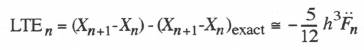   

 

Dividing the right-side of Eq. (8.19) by the integration step size h converts the error per integration step to the error per unit time. For the case where the integrator input F is a sinusoid of frequency  , and the error per unit time becomes  . When divided by F, the result is  , which represents the fractional error in AB-2 integrator transfer function for sinusoidal inputs, as is evident in Eq. (3.36). If we use a central difference formula to approximate   in Eq. (8.19), we obtain the following formula for the local truncation error of the AB-2 integrator:

(8.20)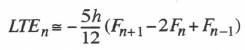   

 

This formula can be computed on-line as part of the real-time simulation. Note that the coefficient 5h/12 in Eq. (8.20) need be calculated only once each integration step, regardless of the number of state variables. Thus the on-line calculation of local truncation error for selected state variables requires only minimal additional arithmetic operations.

 

Figure 8.20 shows plots of the local integration truncation errors, as obtained using the formula in Eq. (8.20), for the simulated airframe output   for multi-rate frame ratios N =10, 8, 6, 4 and 2. Comparison with the global errors in   shown earlier in Figure 8.18 demonstrates that the local truncation errors provide a good indication of the dependence of global airframe simulation errors on the frame-ratio N. The local integration truncation errors in the actuator output  , again calculated on-line using the formula in Eq. (8.20), are shown in Figure 8.21 for N = 10, 8, 6 and 4. Comparison with the global errors previously shown in Figure 8.19 for the same values of N demonstrates that the local truncation errors also provide a good indication of the dependence of actuator simulation global errors on the frame-ratio N. Thus the on-line calculation of local integration truncation errors, which can be accomplished without compromising the integrity of a real-time, hardware-in-the-loop simulation, can be used to select the most desirable frame-ratio N in multi-rate simulations. The local integration truncation error can of course also be used more generally as a tool to determine whether the real-time simulation errors are sufficiently small to satisfy the overall fidelity requirements.

 

8.12 Utilization of Other Integration Algorithms in Multi-rate Integration

All of the example multi-rate simulations considered in this chapter have utilized the AB-2 integration algorithm, which is a second-order predictor method. Although this is the most widely

 

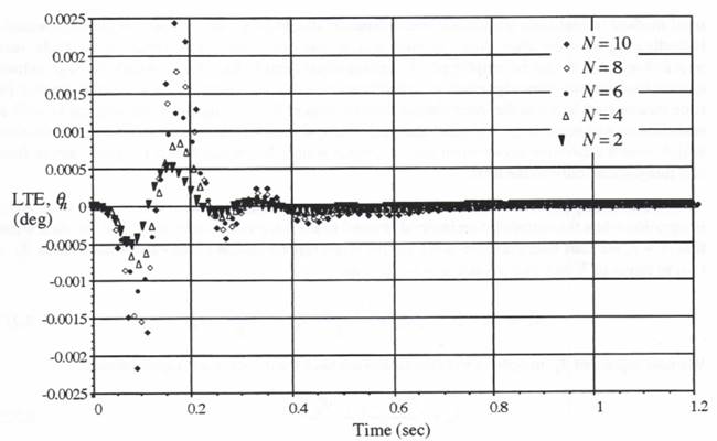
Figure 8.20. Local truncation error in real-time airframe output  for different frame ratios N.

 

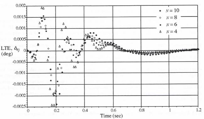
Figure 8.21. Local truncation error in real-time actuator output  for different frame ratios N.

 

used method in real-time simulation, consideration should be given to other integration methods, including higher-order algorithms. In particular, higher-order single-pass predictor methods, such as AB-3 and AB-4, can be employed. Formulas equivalent to Eq. (8.15), which provide extrapolation based on the same algorithm utilized for numerical integration, can be utilized to correct for time mismatches between the input/output data sequences for the multi-rate subsystems as well as real-time input/output data. We recall that such extrapolation formulas eliminate the discontinuities which would otherwise occur when the data upon which the extrapolation is based moves from one integration frame to the next.

 

For example, let us consider the third-order extrapolation algorithm that reduces to AB-3 integration when the extrapolation interval is equal to the integration step size h. For the state equation  , we start with the third-order Taylor series representation of the extrapolated value   at   in terms of X and its derivatives at  . Thus

(8.21)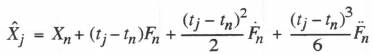   

 

We now represent   to order h with the following backward-difference approximation:

 

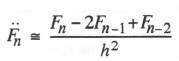
(8.22)

 

 

Next,   is represented with the central-difference approximation   . To

order h², we can then write   as

 

(8.23)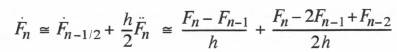   

 

Substituting Eqs. (8.22) and (8.23) into (8.21), we obtain the following third-order extrapolation formula:            

(8.24)

 

In terms of the dimensionless extrapolation interval  , Eq. (8.24) becomes

(8.25)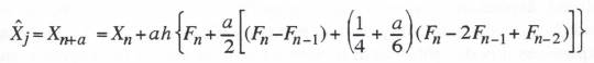   

 

For a = 1, which represents an extrapolation interval   equal to the integration step size h, Eq. (8.25) reduces to  , which is just the formula of Eq. (1.21) for AB-3 integration. Although Eq. (8.24) may appear to be rather complex, the number of required arithmetic operations is not very large for each extrapolation. Thus the term   needs to be calculated only once every integration frame for each state variable and requires but 1 addition. Also, the term   needs to be calculated only once every integration frame and requires only 1 addition, since   where   has been calculated in the previous frame. The extrapolation interval   and the remaining coefficients of   and   need only be calculated once each extrapolation step, regardless of the number of subsystem state variables being extrapolated. It follows that the number of additional calculations required for each implementation of the extrapolation formula given in Eq. (8.24) consists of only 3 additions and 3 multiplications.

 

When multi-pass integration algorithms are used, such as the Runge-Kutta methods or the two-pass Adams-Moulton predictor-corrector methods, it is not possible to select formulas which eliminate extrapolation discontinuities. To illustrate why this is true, we consider the real-time AM-2 predictor-corrector method, which was first introduced in Eqs. (1.29) and (1.30). Here the first pass through the state equations uses predictor integration to compute the state half-way through the integration step h, as shown in Eq. (1.29). Then the second RTAM-2 pass through the state equations is based on the derivative half-way through the frame, as computed from the results of the first pass. This leads to the modified-Euler integration formula given in Eq. (1.30). Thus the RTAM-2 algorithm actually generates two output data sequences, one at half-integer frame times and one at integer frame times. For example, when we apply the RTAM-2 method to the integration of the airframe pitch rate Q to obtain the pitch angle  , we generate two airframe output pitch angle data sequences, one with data points   at the half-integer frame times associated with the predictor pass, and one with data points   at the integer frame times associated with the corrector pass. Similarly, data points for the output pitch rate Q are generated at both half-integer and integer frame times. Designating the half-integer frame time by   and the associated pitch rate by  , we can write the following 2nd-order extrapolation formula, which is the counterpart of Eq. (8.15):

 

After the completion of a predictor pass but before the completion of the corrector pass,   it then follows that   and  . Thus the 2nd-order extrapolation is based on  ,   and  . In this case we note that when the extrapolation interval  , the right side of Eq. (8.26) becomes  , which agrees exactly with the corrector integration formula for  .  On the other hand, after the completion of a corrector pass but before the completion of the next predictor pass,    it then follows that   and  . In this case the extrapolation is based on  ,   and  . Thus Eq. (8.26) represents a 2nd-order extrapolation algorithm that is completely consistent with the RTAM-2 integration method. However, for a single extrapolation time   within a given integration frame, two different extrapolator results for  , can be produced, depending on whether the extrapolation is based on the predictor-pass data points  ,   and   or the corrector-pass data points  ,   and  . From the appropriate Taylor series expansions it is straightforward to derive formulas for the the approximate errors in terms of the dimensionless extrapolation interval  . In this way we find that the error   is equal to   when the extrapolation is based on the predictor-pass data and   when the extrapolation is based on the corrector-pass data. As the dimensionless extrapolation interval a varies between 0 and 1, with the extrapolation based on predictor-pass data for   and corrector-pass data for  , this results in the dimensionless extrapolator error shown in Figure 8.22. In this case the discontinuity occurs at a = 1/2, i.e., half-way through the integration step. Although the shift from predictor-pass data to corrector-pass data can occur at any point inside or outside any particular integration frame in a given multi-rate simulation example, when it occurs within a frame, it is clear that a substantial discontinuity will result. This in turn can add considerable scatter to the extrapolated data sequence outputs compared with the results we have shown thus far in this chapter.

 

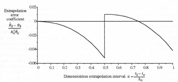
Figure 8.22. Error coefficient for extrapolation based on Eq. (8.25).

 

We therefore conclude that the advantages associated with the use of extrapolation based on the same methodology as that used for numerical integration of the state variables cannot be fully realized when multiple-pass integration methods are used. Thus it appears that single-pass predictor algorithms such as AB-2, AB-3 and AB-4 will in general be more suitable for multi-rate simulation, especially in the real-time case.