7.1 Introduction
We have seen in Chapter 1 that Euler or rectangular integration is the simplest numerical integration algorithm. Because of its simplicity it requires fewer digital instructions to implement and therefore runs faster than any other integration method for a given step size. The big drawback to conventional Euler integration is its poor accuracy. This is because the global truncation errors vary only as the first power of the integration step size.
In this chapter we describe several versions of a modified Euler algorithm which in general requires no more mathematical operations than conventional Euler integration but which exhibits global truncation errors proportional to the square of the integration step size. To introduce the basic algorithm we consider the following two state equations for a velocity vector V and a displacement vector D:
(7.1) ![]()
Here the acceleration vector A is a nonlinear function of D, V, and the input vector U (t). To apply the modified Euler method we represent the velocity vector at half-integer frame times, and the displacement and acceleration vectors at integer frame times. Then the modified Euler difference equations become
(7.2) ![]()
where
(7.3) ![]()
Here h is the integration step size and ![]() represents an estimate of V at the nth frame, since we are only computing V at half-integer frame times. Any of the extrapolation formulas considered in Chapter 4 can be used to compute
represents an estimate of V at the nth frame, since we are only computing V at half-integer frame times. Any of the extrapolation formulas considered in Chapter 4 can be used to compute ![]() . It is evident from Eq. (7.2) that modified Euler integration, as we define it here, is the same as conventional Euler integration, except that the state-variable derivative is defined halfway through the frame instead of at the beginning of the frame. In this regard modified Euler integration is the same algorithm used in the second pass of the real-time RK-2 method in Eqs. (1.27) and (1.28), and the second pass of the RTAM-2 method in Eqs. (1.29) and (1.30).
. It is evident from Eq. (7.2) that modified Euler integration, as we define it here, is the same as conventional Euler integration, except that the state-variable derivative is defined halfway through the frame instead of at the beginning of the frame. In this regard modified Euler integration is the same algorithm used in the second pass of the real-time RK-2 method in Eqs. (1.27) and (1.28), and the second pass of the RTAM-2 method in Eqs. (1.29) and (1.30).
By taking the Z transform of either difference equation in (7.2) using a step size of h/2, we can derive the following formula for the integrator Z transform, ![]() , for modified Euler integration:
, for modified Euler integration:
(7.4) 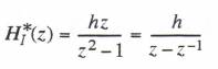
The transfer function for sinusoidal inputs, ![]() , is given by
, is given by
(7.5) 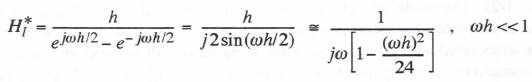
7-1
Comparison of Eq. (7.5) with the standard form of the approximate integrator transfer function ![]() , as first introduced in Eq. (3.37) shows that the integrator error coefficient
, as first introduced in Eq. (3.37) shows that the integrator error coefficient ![]() . This makes the accuracy of modified Euler integration equal to or better than that of any other second-order method, as can be seen by referring to Table 3.1 in Section 3.12. Of course, to realize this accuracy the derivative input halfway through the integration frame must be accurate to order h3. This should be taken into account in the choice of estimation formula when the derivative halfway through the frame is not directly available.
. This makes the accuracy of modified Euler integration equal to or better than that of any other second-order method, as can be seen by referring to Table 3.1 in Section 3.12. Of course, to realize this accuracy the derivative input halfway through the integration frame must be accurate to order h3. This should be taken into account in the choice of estimation formula when the derivative halfway through the frame is not directly available.
7.2 Application to a Second-order Linear System
As a first example we consider the application of the modified Euler method to a second-order linear system described by the state equation
(7.6) ![]()
Here X is the output, U(t) is the input, ![]() is the undamped natural frequency, and
is the undamped natural frequency, and ![]() is the damping ratio. By analogy with Eqs. (7.2) and (7.3) the modified Euler difference equations for the kth integration frame take the following form:
is the damping ratio. By analogy with Eqs. (7.2) and (7.3) the modified Euler difference equations for the kth integration frame take the following form:
(7.7) ![]()
(7.8) ![]()
Note that Eq. (7.7) must be executed first, since the result, ![]() is used in Eq. (7.8). Note also that the estimate for Y at the integer frame k, namely
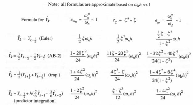
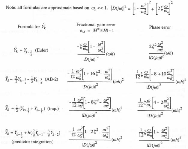
is used in Eq. (7.8). Note also that the estimate for Y at the integer frame k, namely ![]() , must be computed. Table 7.1 lists some candidate formulas for this estimate.
, must be computed. Table 7.1 lists some candidate formulas for this estimate.
Table 7.1
Some Methods for estimating the state ![]() in Modified Euler Integration
in Modified Euler Integration
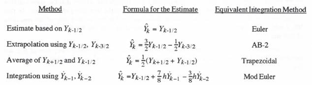
The first formula in Table 7.1 simply replaces ![]() with
with ![]() , the state value at the previous frame time, h(k -1/2). The modified Euler formula for integrating the term
, the state value at the previous frame time, h(k -1/2). The modified Euler formula for integrating the term ![]() in Eq. (7.6) is then equivalent to conventional Euler integration and is so indicated in the table. The global truncation error associated with this portion of the integration will be proportional to
in Eq. (7.6) is then equivalent to conventional Euler integration and is so indicated in the table. The global truncation error associated with this portion of the integration will be proportional to ![]() . In the frequency domain this corresponds to an integrator phase shift of
. In the frequency domain this corresponds to an integrator phase shift of ![]() , as we have seen in Chapter 3. The remaining terms on the right side of Eq. (7.7) will of course be integrated with the full accuracy of the modified Euler method, i.e., integrator gain errors given approximately by
, as we have seen in Chapter 3. The remaining terms on the right side of Eq. (7.7) will of course be integrated with the full accuracy of the modified Euler method, i.e., integrator gain errors given approximately by ![]() . Later we will analyze the effect on the overall simulation accuracy of using Euler integration for the
. Later we will analyze the effect on the overall simulation accuracy of using Euler integration for the ![]() term.
term.
The second formula in Table 7.1 uses linear extrapolation based on ![]() and
and ![]() to compute the estimate
to compute the estimate ![]() . It is easy to see that this is equivalent to using the AB-2 method to integrate the term
. It is easy to see that this is equivalent to using the AB-2 method to integrate the term ![]() on the right side of Eq. (7.7). This leads to an integrator gain error of
on the right side of Eq. (7.7). This leads to an integrator gain error of ![]() , again based on our results in Chapter 3. Although this error is proportional to h2, it is still 10 times larger than the gain error associated with the modified Euler method, which will therefore degrade somewhat the accuracy of the overall simulation.
, again based on our results in Chapter 3. Although this error is proportional to h2, it is still 10 times larger than the gain error associated with the modified Euler method, which will therefore degrade somewhat the accuracy of the overall simulation.
The third formula in Table 7.1 uses the average of ![]() and
and ![]() to compute the estimate
to compute the estimate ![]() . This is equivalent to trapezoidal integration and leads to an approximate gain error of
. This is equivalent to trapezoidal integration and leads to an approximate gain error of ![]() in integrating the term
in integrating the term ![]() on the right side of Eq. (7.7). In this case
on the right side of Eq. (7.7). In this case ![]() appears on both sides of Eq. (7.7), which then becomes an implicit equation. However, in our example here the equation is linear and we can easily solve it to produce an explicit formula for
appears on both sides of Eq. (7.7), which then becomes an implicit equation. However, in our example here the equation is linear and we can easily solve it to produce an explicit formula for ![]() . If the right side of Eq. (7.7) involves a nonlinear function of Y, it may still be possible to generate an approximate explicit formula for
. If the right side of Eq. (7.7) involves a nonlinear function of Y, it may still be possible to generate an approximate explicit formula for ![]() through a linearization procedure, as we shall see in a later example in this chapter.
through a linearization procedure, as we shall see in a later example in this chapter.
The final formula in Table 7.1 is based on a predictor integration method using ![]() and
and ![]() . The error associated with the calculation of the estimate
. The error associated with the calculation of the estimate ![]() is then the local truncation error associated with the integration formula. This error will be proportional to h3, which means that
is then the local truncation error associated with the integration formula. This error will be proportional to h3, which means that ![]() will be equal to
will be equal to ![]() to order h2. In this case the asymptotic errors associated with the integration of the term
to order h2. In this case the asymptotic errors associated with the integration of the term ![]() in Eq. (7.7) will be the same as those for ideal modified Euler integration, and the best overall simulation accuracy will in general be obtained.
in Eq. (7.7) will be the same as those for ideal modified Euler integration, and the best overall simulation accuracy will in general be obtained.
In the sections that follow we will analyze the accuracy of the modified Euler simulation of the second-order system described by Eq. (7.6) by considering transfer function errors and characteristic root errors. This in turn will lead us to general results for the modified Euler method. We will also consider the stability region in the ![]() plane when using the various formulas in Table 7.1 for estimating
plane when using the various formulas in Table 7.1 for estimating ![]() .
.
7.3 Accuracy Analysis Using Integrator Transfer Function Models
When any of the first three formulas in Table 7.1 are used to compute ![]() in Eq. (7.7), the resulting simulation will involve two different integration methods, namely, modified Euler and a second method, as listed in the third column in the table. We have already seen in Eq. (3.37) of Chapter 3 that the transfer function of single-pass (or equivalent single-pass) integrators can be written approximately as
in Eq. (7.7), the resulting simulation will involve two different integration methods, namely, modified Euler and a second method, as listed in the third column in the table. We have already seen in Eq. (3.37) of Chapter 3 that the transfer function of single-pass (or equivalent single-pass) integrators can be written approximately as
(7.9) 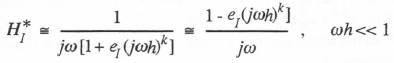
Using Eq. (7.9) to model each integration in the numerical simulation, we can determine the approximate frequency-domain representation of the simulation itself, from which the transfer function errors can be determined. Letting ![]() for modified Euler integration and
for modified Euler integration and ![]() for the method used to integrate the term
for the method used to integrate the term ![]() we can rewrite Eq. (7.6) in the frequency domain as
we can rewrite Eq. (7.6) in the frequency domain as
(7.10) 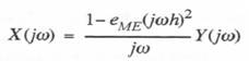
and
(7.11) 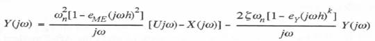
Here the order of the modified Euler method is 2 and the order of the alternative method is k. By eliminating ![]() from Eqs. (7.10) and (7.11), we can solve for the digital system transfer function,
from Eqs. (7.10) and (7.11), we can solve for the digital system transfer function, ![]() . In this way we obtain
. In this way we obtain

(7.12)
For ![]() Eq. (7.12) reduces to the formula for the ideal second-order system transfer function. Thus
Eq. (7.12) reduces to the formula for the ideal second-order system transfer function. Thus
(7.13) 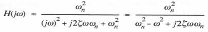
The transfer function H(s) of the continuous system is obtained by simply replacing ![]() with s. The poles of H(s) are the characteristic roots
with s. The poles of H(s) are the characteristic roots ![]() of the continuous system. For the ideal second-order linear system these are the roots of the characteristic equation
of the continuous system. For the ideal second-order linear system these are the roots of the characteristic equation ![]() and are given by
and are given by
(7.14) ![]()
In the same way, to obtain the approximate formulas for the characteristic roots ![]() of the digital system we replace
of the digital system we replace ![]() with
with ![]() in Eq. (7.12) and set the denominator equal to zero. Thus the characteristic equation becomes
in Eq. (7.12) and set the denominator equal to zero. Thus the characteristic equation becomes
(7.15) ![]()
Multiplying by ![]() and neglecting terms in e2, we can rewrite Eq. (7.15) as
and neglecting terms in e2, we can rewrite Eq. (7.15) as
(7.16) ![]()
For the case where ![]() in Eq. (7.7) is estimated by any of the bottom three methods in Table 7.1, the order of the effective method used to integrate the term
in Eq. (7.7) is estimated by any of the bottom three methods in Table 7.1, the order of the effective method used to integrate the term ![]() in Eq. (7.6) is given by k = 2. Under these conditions the digital system roots
in Eq. (7.6) is given by k = 2. Under these conditions the digital system roots ![]() will be equal to the continuous-system roots
will be equal to the continuous-system roots ![]() to order h2. It follows that
to order h2. It follows that ![]() or
or ![]() to order h2. Making this substitution for
to order h2. Making this substitution for ![]() in the integrator error terms in Eq. (7.16), we obtain the following equation, which is accurate to order h2:
in the integrator error terms in Eq. (7.16), we obtain the following equation, which is accurate to order h2:
(7.17) ![]()
Multiplication by ![]() results in the following equation for the characteristic roots, which again is accurate to order h2:
results in the following equation for the characteristic roots, which again is accurate to order h2: ![]()
(7.18)
From the definition of the undamped natural frequency ![]() and damping ratio
and damping ratio ![]() of the digital system, the characteristic equation for the digital roots
of the digital system, the characteristic equation for the digital roots ![]() is given by
is given by
(7.19) ![]()
Comparison of Eqs. (7.18) and (7.19) shows that ![]() from which we can solve for
from which we can solve for ![]() the fractional error in undamped natural frequency. Thus to order h2
the fractional error in undamped natural frequency. Thus to order h2
(7.20) 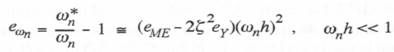
Equating the middle terms on the left side of Eqs. (7.18) and (7.19) and using Eq. (7.20) for ![]() , we obtain the following formula for the damping ratio error
, we obtain the following formula for the damping ratio error ![]() to order h2:
to order h2:
(7.21) ![]()
The fractional error in damped frequency, ![]() is given by
is given by
(7.22)
As noted earlier, Eqs. (7.20), (7.21) and (7.22) represent approximate formulas for the undamped natural frequency, damping ratio, and damped frequency errors when simulating a second-order linear system with modified Euler integration (error coefficient ![]() ) , but with a different second-order integration method (error coefficient
) , but with a different second-order integration method (error coefficient ![]() ) for the damping term. For the case where we use the conventional Euler method to integrate the
) for the damping term. For the case where we use the conventional Euler method to integrate the ![]() term in Eq. (7.6), i.e., the first method in Table 7.1,
term in Eq. (7.6), i.e., the first method in Table 7.1, ![]() and k = 1. To first order in h Eq. (7.15) can then be written as
and k = 1. To first order in h Eq. (7.15) can then be written as
(7.23)
Comparison with Eq. (7.19) yields the following approximate error formulas when conventional Euler integration ![]() is used for the damping term:
is used for the damping term:
(7.24) 
Here all three error formulas depend on the first power of the step size h. However, as the damping ratio ![]() approaches zero, the first-order errors vanish and the errors become second-order in h. In fact, it can be shown that when
approaches zero, the first-order errors vanish and the errors become second-order in h. In fact, it can be shown that when ![]() , the modified Euler simulation of the second-order system represented by Eq. (7.6) exhibits exactly zero damping, regardless of the step size h. This suggests that the method may be particularly effective in simulating lightly-damped systems.
, the modified Euler simulation of the second-order system represented by Eq. (7.6) exhibits exactly zero damping, regardless of the step size h. This suggests that the method may be particularly effective in simulating lightly-damped systems.
For each of the damping-term estimation formulas given in Table 7.1, Table 7.2 lists the asymptotic formulas for the characteristic-root frequency and damping errors. The formulas are based on Eqs. (7.20), (7.21), (7.22) and (7.24) with ![]() for modified Euler integration and
for modified Euler integration and ![]() 5/12 and -1/12 for Euler, AB-2 and trapezoidal integration, respectively. As expected, the table shows that the damping ratio and frequency errors for finite
5/12 and -1/12 for Euler, AB-2 and trapezoidal integration, respectively. As expected, the table shows that the damping ratio and frequency errors for finite ![]() are the smallest when predictor integration is used to calculate
are the smallest when predictor integration is used to calculate ![]() in Eq. (7.7). When
in Eq. (7.7). When ![]() , the damping ratio error vanishes, and the approximate fractional error in frequency becomes
, the damping ratio error vanishes, and the approximate fractional error in frequency becomes ![]() for all four methods.
for all four methods.
Table 7.2
Root Frequency and Damping Ratio Errors for Various Methods of Estimating ![]() for the Damping Term in Modified Euler Integration
for the Damping Term in Modified Euler Integration
We turn next to the consideration of the transfer function errors. For the lower three methods in Table 7.1 the order of the effective method used to integrate the damping term ![]() is given by k = 2. In this case Eq. (7.12) for
is given by k = 2. In this case Eq. (7.12) for ![]() can be written as
can be written as
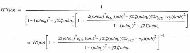
where ![]() is the continuous system transfer function given earlier in Eq. (7.13). It follows that the fractional error in transfer function is given approximately by
is the continuous system transfer function given earlier in Eq. (7.13). It follows that the fractional error in transfer function is given approximately by
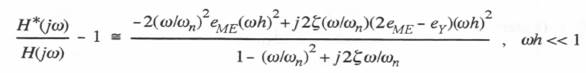
(7.25)
After rationalization, we obtain the following formulas for the fractional gain error and the phase error from the real and imaginary parts, respectively, of H*/H – 1:
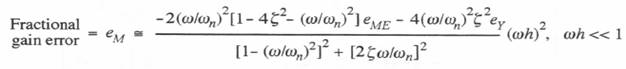 (7.26)
(7.27) 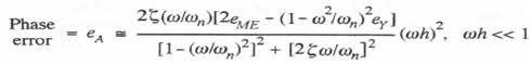
For the case where Euler integration is, in effect, used for integrating the damping term (the first method shown in Table 7.1), ![]() and k = 1 in Eq. (7.12). Also, to first order in h the terms involving
and k = 1 in Eq. (7.12). Also, to first order in h the terms involving ![]() vanish, and the following approximate formulas for the transfer function fractional gain error and the phase error are easily derived:
vanish, and the following approximate formulas for the transfer function fractional gain error and the phase error are easily derived:

(7.28)
For each of the damping-term estimation formulas given in Table 7.1, Table 7.3 lists the asymptotic formulas for the transfer function gain and phase errors. The formulas are based on Eqs. (7.26), (7.27) and (7.28) with ![]() for modified Euler integration and
for modified Euler integration and ![]() = 5/12, -1/12 and 1/24 for AB-2, trapezoidal and predictor integration, respectively. As in the case of the characteristic root errors of Table 7.2, Table 73 shows that the transfer function gain and phase errors for finite
= 5/12, -1/12 and 1/24 for AB-2, trapezoidal and predictor integration, respectively. As in the case of the characteristic root errors of Table 7.2, Table 73 shows that the transfer function gain and phase errors for finite ![]() are the smallest when predictor integration is used to calculate
are the smallest when predictor integration is used to calculate ![]() in Eq. (7.7). Again, this is to be expected, since the integrator error coefficient for predictor integration is smaller than the error coefficient for either AB-2 or trapezoidal integration.
in Eq. (7.7). Again, this is to be expected, since the integrator error coefficient for predictor integration is smaller than the error coefficient for either AB-2 or trapezoidal integration.
Table 7.3
Transfer Function Gain and Phase Errors for Various Methods of Estimating ![]() for the Damping Term in Modified Euler Integration
for the Damping Term in Modified Euler Integration
7.4 Time Domain Errors
In Chapter 3, Section 3.13, we found it useful to compare the performance of different integration methods in the time domain, in addition to considering characteristic root and transfer function errors. In this section we consider the response of the second-order linear system, as simulated with modified Euler integration, to the same acceleration-limited step input used in Section 3.13. As shown in Figure 3.14, this input avoids the discontinuity in displacement inherent in a true step input and yet can produce a response quite similar to the ideal step response. In this way we avoid the domination of errors caused by input discontinuities when using predictor integration algorithms. From Eq. (3.176) we recall that the acceleration-limited step input U(t) is given by
(7.29) 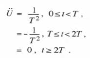
When integrated twice with T set equal to ![]() , Eq. (3.29) yields the input U(t) shown in Figure 3.14. We consider the simulated response of the second-order system using the modified Euler difference equations (7.7) and (7.8) with the damping ratio
, Eq. (3.29) yields the input U(t) shown in Figure 3.14. We consider the simulated response of the second-order system using the modified Euler difference equations (7.7) and (7.8) with the damping ratio ![]() , which is the same value used earlier in Figure 3.14. Here we will plot the respective solution errors when the velocity estimate
, which is the same value used earlier in Figure 3.14. Here we will plot the respective solution errors when the velocity estimate ![]() , as needed in the modified Euler mechanization, is calculated using each of the bottom three formulas in Table 7.1.
, as needed in the modified Euler mechanization, is calculated using each of the bottom three formulas in Table 7.1.
For the case where ![]() is computed as the average of
is computed as the average of ![]() and
and ![]() , as shown in the third formula in Table 7.1, Eq. (7.7) becomes implicit in
, as shown in the third formula in Table 7.1, Eq. (7.7) becomes implicit in ![]() . Since the equation is linear, however, we can solve for
. Since the equation is linear, however, we can solve for ![]() , which results in the following difference equation:
, which results in the following difference equation:
(7.30) ![]()
where
(7.31) 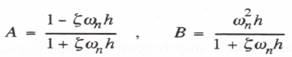
For a dimensionless integration step size given by ![]() , Figure 7.1 shows the error in simulated response to the acceleration limited step input. In addition to the results when using each of the last three formulas in Table 7.1 for
, Figure 7.1 shows the error in simulated response to the acceleration limited step input. In addition to the results when using each of the last three formulas in Table 7.1 for ![]() , Figure 7.1 also shows the results when conventional AB-2 integration is used. The superiority of all three versions of the modified Euler method is clearly evident. Not shown are the results when the estimate
, Figure 7.1 also shows the results when conventional AB-2 integration is used. The superiority of all three versions of the modified Euler method is clearly evident. Not shown are the results when the estimate ![]() , which is equivalent to Euler integration of the damping term, as noted in the first entry in Table 7.1. In this case the errors are proportional to h rather than h2 for finite
, which is equivalent to Euler integration of the damping term, as noted in the first entry in Table 7.1. In this case the errors are proportional to h rather than h2 for finite ![]() which is the case here. As a result, the errors are even larger than those shown in Figure 7.1 for conventional AB-2 integration. Clearly the modified Euler method that employs second-order predictor integration to compute
which is the case here. As a result, the errors are even larger than those shown in Figure 7.1 for conventional AB-2 integration. Clearly the modified Euler method that employs second-order predictor integration to compute ![]() exhibits the smallest error. This is to be expected based on our previous results in Tables 7.2 and 73.
exhibits the smallest error. This is to be expected based on our previous results in Tables 7.2 and 73.
7.5 Stability of Modified Euler Methods
We have seen that the stability of integration algorithms often represents as important a consideration as accuracy when simulating dynamic systems. To study the stability of the modified-Euler methods considered here, we start by determining the Z transform, ![]() for each of the schemes listed in Table 7.1. For example, consider the case where the estimate
for each of the schemes listed in Table 7.1. For example, consider the case where the estimate ![]() , which is equivalent to Euler integration of the damping term. Then Eqs. (7.7) and (7.8) lead to the following Z transform:
, which is equivalent to Euler integration of the damping term. Then Eqs. (7.7) and (7.8) lead to the following Z transform:
(7.32) 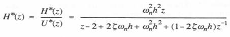
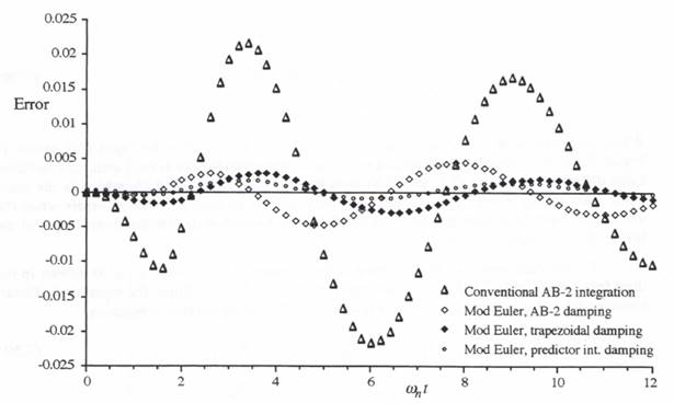
Figure 7.1. Acceleration-limited unit-step response errors for different versions of modified-Euler integration compared with conventional AB-2 integration; ![]() .
.
We recall that the stability boundary in the ![]() plane is determined by setting the denominator of H*(z) equal to zero with
plane is determined by setting the denominator of H*(z) equal to zero with ![]() , i.e.,
, i.e., ![]() , which corresponds to neutral stability. When we let
, which corresponds to neutral stability. When we let ![]() both the real and imaginary parts of the denominator must vanish. Here the imaginary part is equal to
both the real and imaginary parts of the denominator must vanish. Here the imaginary part is equal to ![]() , which in general will only vanish when
, which in general will only vanish when ![]() . . We conclude that
. . We conclude that ![]() or
or ![]() , which corresponds to z = 1 or -1, respectively. For z = 1, the denominator of H*(z) becomes
, which corresponds to z = 1 or -1, respectively. For z = 1, the denominator of H*(z) becomes ![]() and it follows that
and it follows that ![]() , a trivial solution. For z = -1, the denominator of H*(z) becomes
, a trivial solution. For z = -1, the denominator of H*(z) becomes ![]() which, when set equal to zero, results in the following formula for
which, when set equal to zero, results in the following formula for ![]() :
:
(7.33) ![]()
From Eq. (7.14) for ![]() in terms of
in terms of ![]() and
and ![]() we obtain the following formula for the stability boundary in the
we obtain the following formula for the stability boundary in the ![]() plane when the modified Euler integration method is used with conventional Euler to integrate the damping term:
plane when the modified Euler integration method is used with conventional Euler to integrate the damping term:
(7.34) 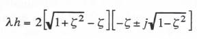
A similar approach is used to obtain the stability boundary in the ![]() plane for the other modified Euler schemes in Table 7.1. The resulting formulas are summarized in Table 7.4. In each case neutral stability occurs for z = -1, which corresponds to an undamped oscillation at one-half the integration frame rate 1/h.
plane for the other modified Euler schemes in Table 7.1. The resulting formulas are summarized in Table 7.4. In each case neutral stability occurs for z = -1, which corresponds to an undamped oscillation at one-half the integration frame rate 1/h.
Table 7.4
![]() Plane Stability Boundary Formulas for Various Methods of Estimating
Plane Stability Boundary Formulas for Various Methods of Estimating ![]() for the Damping Term in Modified Euler Integration
for the Damping Term in Modified Euler Integration
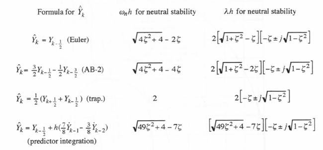
The actual stability boundaries are shown in Figure 7.2. In addition to the four modified Euler methods considered here, Figure 7.2 also shows for reference purposes the stability boundary for AB-2 integration, the most widely used of the real-time algorithms. As is customary, only the upper half of the stability regions is shown, since the boundaries are all symmetric with respect to the real axis. Clearly the scheme which bases the estimate for ![]() on the average of
on the average of ![]() and
and ![]() , equivalent to trapezoidal integration of the damping term, has by far the largest stability region of all the modified Euler methods. On the other hand, the scheme which bases the estimate for
, equivalent to trapezoidal integration of the damping term, has by far the largest stability region of all the modified Euler methods. On the other hand, the scheme which bases the estimate for ![]() on second-order predictor integration exhibits the smallest of the modified Euler stability regions. The right hand boundary for all the modified Euler methods is the imaginary axis. As noted earlier, this means that the modified Euler algorithm exhibits exactly zero damping, regardless of integration step size, when used to simulate an undamped second-order system. It is also apparent that the modified Euler methods in general are more robust in stability than AB-2 integration when the system being simulated is lightly damped.
on second-order predictor integration exhibits the smallest of the modified Euler stability regions. The right hand boundary for all the modified Euler methods is the imaginary axis. As noted earlier, this means that the modified Euler algorithm exhibits exactly zero damping, regardless of integration step size, when used to simulate an undamped second-order system. It is also apparent that the modified Euler methods in general are more robust in stability than AB-2 integration when the system being simulated is lightly damped.
It should be noted that all of the modified Euler methods considered here are equally applicable to nonlinear systems with the exception of the scheme which effectively uses trapezoidal integration for the damping term. In the trapezoidal case, when the system being simulated is linear, we are able to solve the resulting implicit equation to produce an explicit formula. Eqs. (7.30) and (7.31) provide an example. Of course, this is not in general possible when the time derivative of the velocity Y is a nonlinear function of Y. Even in this case, however, it may be possible to obtain either an exact or at least an approximately exact explicit formula, as we shall see in the next section. In this way we can take advantage of the quite large stability region associated with modified Euler integration when using the trapezoidal method to integrate the Y – dependent terms.
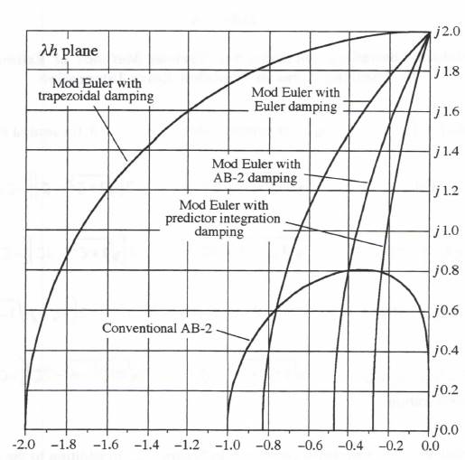
Figure 7.2. Stability boundaries for various versions of modified-Euler integration compared with conventional AB-2 integration.
7.6 Application to a Nonlinear System
We now consider the use of modified Euler integration to simulate a nonlinear system. For simplicity we choose the same second-order system described earlier in Section (7.6), but with a quadratic rather than linear damping term. The two state equations are given by
(7.35) ![]()
The magnitude of the damping term is clearly proportional to ![]() , but the polarity is that of the velocity, Y. As a specific example we let the quadratic damping constant C = 1. We also utilize the same acceleration-limited unit step input given in Eq. (7.29) with
, but the polarity is that of the velocity, Y. As a specific example we let the quadratic damping constant C = 1. We also utilize the same acceleration-limited unit step input given in Eq. (7.29) with ![]() and
and ![]() . With zero initial conditions the exact response is shown in Figure 7.3. Also shown in the figure is the response of the linear system with
. With zero initial conditions the exact response is shown in Figure 7.3. Also shown in the figure is the response of the linear system with ![]() . The effect of the quadratic damping is to make the transient die out more slowly as the amplitude of the transient decays.
. The effect of the quadratic damping is to make the transient die out more slowly as the amplitude of the transient decays.
The solution errors in simulating the second-order system with quadratic damping using the various modified Euler schemes are shown in Figure 7.4. Also shown is the result when conventional AB-2 integration is used. The modified Euler methods are clearly superior. Again, the
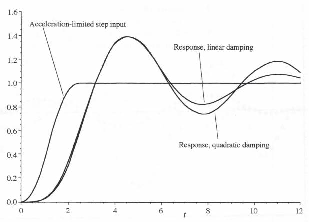
Figure 7.3. Acceleration-limited step response of second-order systems with linear and quadratic damping.
scheme in Table 7.1 which uses second-order predictor integration to calculate the estimate ![]() , gives the best performance. In mechanizing the method in Table 7.1 which computes
, gives the best performance. In mechanizing the method in Table 7.1 which computes ![]() based on the average of
based on the average of ![]() and
and ![]() , we have approximated
, we have approximated ![]() with
with ![]() . Thus the difference equation for simulating (7.35) becomes
. Thus the difference equation for simulating (7.35) becomes
(7.36) ![]()
and we can solve explicitly for ![]() to obtain
to obtain
(7.37) 
Eqs. (7.37) and (7.8) were used to obtain the simulation results labelled “Mod Euler, trapezoidal damping” in Figure 7.4.
In general, of course, the right-hand side of the state equation for ![]() may not be as simple a nonlinear function of the velocity Y as the quadratic form in Eq. (7.35), where we were able to replace
may not be as simple a nonlinear function of the velocity Y as the quadratic form in Eq. (7.35), where we were able to replace ![]() with the approximation
with the approximation ![]() . However, in the general case it is possible to represent the nonlinear functionF(Y) with the following first-order approximation:
. However, in the general case it is possible to represent the nonlinear functionF(Y) with the following first-order approximation:
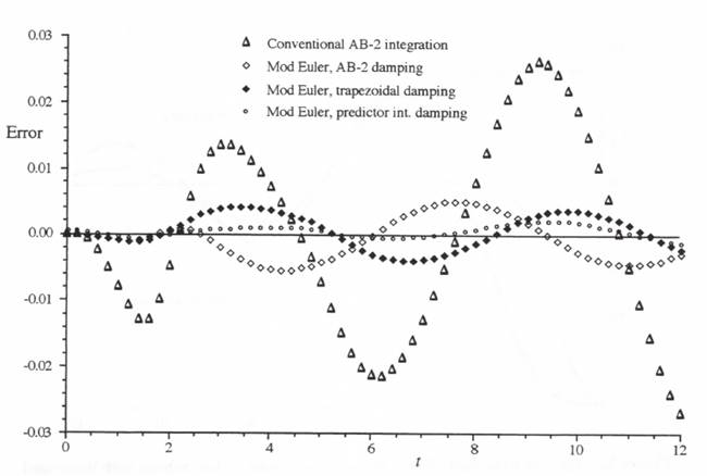
Figure 7.4. Acceleration-limited step-response errors in simulating a second-order system with quadratic damping using modified-Euler integration.
(7.38) 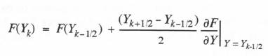
Since the right side of Eq. (7.38) is a linear function of ![]() , the modified Euler difference equation
, the modified Euler difference equation ![]() can now be solved explicitly for
can now be solved explicitly for ![]() . In fact, when equation (7.38) is applied to the quadratic damping function,
. In fact, when equation (7.38) is applied to the quadratic damping function, ![]() , it results directly in the approximation
, it results directly in the approximation ![]() , as used above in Eq. (7.36). Thus Eq. (7.38) provides a general approach to using the equivalent of trapezoidal integration for Y-dependent nonlinear functions in the state equation for Y. In this way we can take advantage of the improved stability of this version of modified Euler integration, as exhibited in Figure 7.2. However, if stability is not a problem, the approach which calculates the approximation
, as used above in Eq. (7.36). Thus Eq. (7.38) provides a general approach to using the equivalent of trapezoidal integration for Y-dependent nonlinear functions in the state equation for Y. In this way we can take advantage of the improved stability of this version of modified Euler integration, as exhibited in Figure 7.2. However, if stability is not a problem, the approach which calculates the approximation ![]() using predictor integration can always be used and in general produces the most accurate result, as we have seen in our examples here .
using predictor integration can always be used and in general produces the most accurate result, as we have seen in our examples here .
7.7 Modified Euler Integration with Root Matching
In this section we determine the improvements in modified Euler simulation of second-order linear systems that can be made using characteristic-root matching. Consider first the case in Table 7.1 where we let ![]() , equivalent to Euler integration of the damping term in Eq. 7.6.
, equivalent to Euler integration of the damping term in Eq. 7.6.
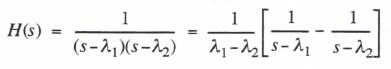
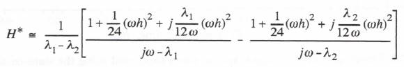
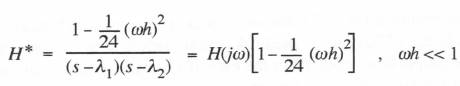
The Z transform, H*(z), of the resulting digital system when the remaining integrations use modified Euler integration, has already been presented in Eq. (7.32). The roots z1 and z2 of the denominator of H*(z) are given by the formula
(7.39) ![]()
We have seen in Eq. (2.14) that the corresponding characteristic roots, ![]() , of the digital system are related to the z-transform poles, z1.2 , by the formulas
, of the digital system are related to the z-transform poles, z1.2 , by the formulas
(7.40) ![]()
The damping ratio ![]() and the undamped natural frequency
and the undamped natural frequency ![]() of the digital system are related to the digital system characteristic roots,
of the digital system are related to the digital system characteristic roots, ![]() , by the following formulas:
, by the following formulas:
(7.41) 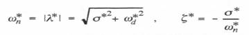
From Eqs. (7.39), (7.40) and (7.41) we can determine the exact formulas for ![]() and
and ![]() for the modified Euler simulation in terms of
for the modified Euler simulation in terms of ![]() and
and ![]() for the original continuous system. From Eq. (7.39) for
for the original continuous system. From Eq. (7.39) for ![]() we find that
we find that ![]() . Thus
. Thus ![]() and the digital simulation will have zero damping for any step-size h within the range
and the digital simulation will have zero damping for any step-size h within the range ![]() . For the case of finite damping the exact formulas reduce to the asymptotic formulas in Eq. (7.24) when
. For the case of finite damping the exact formulas reduce to the asymptotic formulas in Eq. (7.24) when ![]() .
.
From Eqs. (7.39), (7.40) and (7.41) we can also solve for ![]() and
and ![]() in terms of
in terms of ![]() and
and ![]() . The resulting formulas allow us to calculate
. The resulting formulas allow us to calculate ![]() and
and ![]() for the original continuous system, given
for the original continuous system, given ![]() and
and ![]() for the digital system. If in these formulas we replace
for the digital system. If in these formulas we replace ![]() and
and ![]() with
with ![]() and
and ![]() , respectively, and then replace
, respectively, and then replace ![]() and
and ![]() with
with ![]() and
and ![]() , respectively, we obtain the following formulas:
, respectively, we obtain the following formulas:
(7.42) ![]()
(7.43) 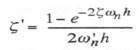
These formulas permit us to calculate the parameters ![]() and
and ![]() which, when used in the modified Euler difference equations, will make the digital simulation match exactly the specified undamped natural frequency
which, when used in the modified Euler difference equations, will make the digital simulation match exactly the specified undamped natural frequency ![]() and damping ratio
and damping ratio ![]() . The new difference equations can be rewritten as
. The new difference equations can be rewritten as
(7.44) ![]()
(7.45) ![]()
(7.46) 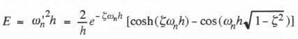
The digital simulation using Eqs. (7.44), (7.45) and (7.46) will yield a solution for which ![]() and
and ![]() . Thus the characteristic roots of the digital simulation will match exactly the characteristic roots of the continuous system being simulated.
. Thus the characteristic roots of the digital simulation will match exactly the characteristic roots of the continuous system being simulated.
Next, we determine the transfer function errors when the above root-matching procedure is used. From Eqs. (7.42) and (7.43) we can derive the following approximate equations for ![]() and
and ![]() .
.
(7.47) ![]()
(7.48) ![]()
We now substitute ![]() and
and ![]() , as given above, along with the power series representation of
, as given above, along with the power series representation of ![]() , into Eq. (7.32) to obtain the following asymptotic formulas for the transfer function gain and phase errors:
, into Eq. (7.32) to obtain the following asymptotic formulas for the transfer function gain and phase errors:
(7.49) ![]()
Note that both errors depend on h2 instead of h, as in the corresponding formulas in Eq. (7.28) when root matching is not employed.
The same root matching technique can be applied to the modified Euler method which computes ![]() as the average of
as the average of ![]() and
and ![]() , as shown in the third formula in Table 7.1. From the Z transform of the digital system represented by Eqs. (7.30), (7.31) and (7.8) we can determine the exact formulas for
, as shown in the third formula in Table 7.1. From the Z transform of the digital system represented by Eqs. (7.30), (7.31) and (7.8) we can determine the exact formulas for ![]() and
and ![]() . Again, these formulas permit us to calculate
. Again, these formulas permit us to calculate ![]() and
and ![]() for the original continuous system, given
for the original continuous system, given ![]() and
and ![]() for the digital system. Following the same procedure used above when Euler rather than trapezoidal integration is used for the damping term, we replace
for the digital system. Following the same procedure used above when Euler rather than trapezoidal integration is used for the damping term, we replace ![]() and
and ![]() with
with ![]() and
and ![]() , respectively, followed by the replacement of
, respectively, followed by the replacement of ![]() and
and ![]() with
with ![]() and
and ![]() , respectively. This leads directly to the same difference equation given above in Eq. (7.44), with the coefficients for D and E again given by Eqs. (7.45) and (7.46). Thus it makes no difference whether
, respectively. This leads directly to the same difference equation given above in Eq. (7.44), with the coefficients for D and E again given by Eqs. (7.45) and (7.46). Thus it makes no difference whether ![]() is approximated with
is approximated with ![]() or the average of
or the average of ![]() and
and ![]() ; the modified Euler difference equations are identical when root matching is used. It follows that the transfer function
; the modified Euler difference equations are identical when root matching is used. It follows that the transfer function ![]() is the same and the approximation formulas given in Eq. (7.49) also apply.
is the same and the approximation formulas given in Eq. (7.49) also apply.
Note in Eq. (7.49) that the fractional error in gain, ![]() , is completely independent of the damping ratio
, is completely independent of the damping ratio ![]() , and the phase error
, and the phase error ![]() approaches zero as
approaches zero as ![]() approaches zero. Thus the modified-Euler method with matched roots will be especially effective in simulating lightly-damped second-order systems, such as in the representation of structural modes. This is illustrated in the example shown in Figure 7.5, where gain and phase versus frequency for a second-order system with
approaches zero. Thus the modified-Euler method with matched roots will be especially effective in simulating lightly-damped second-order systems, such as in the representation of structural modes. This is illustrated in the example shown in Figure 7.5, where gain and phase versus frequency for a second-order system with ![]() are shown. Because of the sharp resonant peak in gain and the extremely rapid change in phase as
are shown. Because of the sharp resonant peak in gain and the extremely rapid change in phase as ![]() passes through
passes through ![]() , it is very critical that both the natural frequency and damping ratio of the digital simulation match that of the continuous system. The table at the bottom of the figure lists the transfer function errors for input frequencies in the vicinity of
, it is very critical that both the natural frequency and damping ratio of the digital simulation match that of the continuous system. The table at the bottom of the figure lists the transfer function errors for input frequencies in the vicinity of ![]() for the specific case of
for the specific case of ![]() , which corresponds to only 2 integration steps per radian or 12.57 steps per cycle. Shown in the table are the gain and phase errors based on both an exact calculation using the system Z transform and also the approximate formulas of Eq. (7.49). Note how closely the approximate calculations agree with the exact, even for the example here for which
, which corresponds to only 2 integration steps per radian or 12.57 steps per cycle. Shown in the table are the gain and phase errors based on both an exact calculation using the system Z transform and also the approximate formulas of Eq. (7.49). Note how closely the approximate calculations agree with the exact, even for the example here for which ![]() .
.
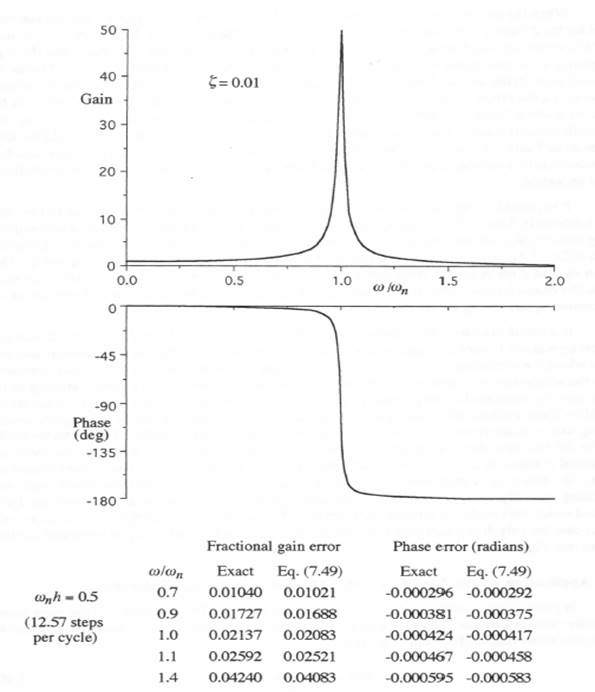
Figure 7.5. Frequency response of lightly-damped second-order system using modified-Euler integration with root matching, ![]() .
.
When the transfer function errors in Table 7.3 for the case where trapezoidal integration is used for the damping term are compared with the gain and phase errors in Eq. (7.48), it is evident that the errors are much smaller in the latter case when the damping ratio is small and the input frequency ![]() is approximately equal to
is approximately equal to ![]() . This occurs because, under these conditions, the denominators in the gain and phase error formulas in Table 73 become small. On the other hand, for
. This occurs because, under these conditions, the denominators in the gain and phase error formulas in Table 73 become small. On the other hand, for ![]() the errors represented in Table 7.3 are much smaller than those in Eq. (7.48). In this case the modified Euler algorithm which uses root matching is less favorable. For
the errors represented in Table 7.3 are much smaller than those in Eq. (7.48). In this case the modified Euler algorithm which uses root matching is less favorable. For ![]() both methods yield the same gain and phase errors. Thus the choice of one of the modified Euler methods in Table 7.3 without root matching or, alternatively, a method utilizing the root matching introduced in this section, depends on the input frequency regime over which accurate simulation is most important.
both methods yield the same gain and phase errors. Thus the choice of one of the modified Euler methods in Table 7.3 without root matching or, alternatively, a method utilizing the root matching introduced in this section, depends on the input frequency regime over which accurate simulation is most important.
It is possible to extend the root-matching technique described in this section to the other two schemes in Table 7.1, namely the use of either linear extrapolation or second-order predictor integration to calculate the estimate ![]() , as needed for the damping term in the modified Euler formula of Eq. (7.7). In each case formulas can be derived for
, as needed for the damping term in the modified Euler formula of Eq. (7.7). In each case formulas can be derived for ![]() and
and ![]() in terms of
in terms of ![]() and
and ![]() . Then when
. Then when ![]() and
and ![]() are replaced, respectively, by
are replaced, respectively, by ![]() and
and ![]() in the modified Euler difference equations, the characteristic roots of the resulting simulation will agree exactly with the roots of the continuous system being simulated.
in the modified Euler difference equations, the characteristic roots of the resulting simulation will agree exactly with the roots of the continuous system being simulated.
It is useful to examine the time-domain performance of the modified Euler method with root matching when it is used to simulate the second-order system with the acceleration-limited step input which we considered earlier in Section 7.4. Figure 7.6 shows the resulting errors compared with the solution errors obtained for the two most accurate schemes when root matching is not used, namely, trapezoidal-integration damping and predictor-integration damping. Whereas the modified Euler method which uses predictor integration to compute ![]() exhibits a slightly smaller startup transient, the error for the root matching method damps more rapidly. This is undoubtedly due to the fact that there is no error caused by a frequency difference between the ideal and numerical transient in the case of root matching, since by definition the transient frequencies are the same. It should be remembered, however, that the modified Euler method which uses root matching can only be applied to the simulation of linear systems, whereas the modified Euler method which uses predictor integration to compute
exhibits a slightly smaller startup transient, the error for the root matching method damps more rapidly. This is undoubtedly due to the fact that there is no error caused by a frequency difference between the ideal and numerical transient in the case of root matching, since by definition the transient frequencies are the same. It should be remembered, however, that the modified Euler method which uses root matching can only be applied to the simulation of linear systems, whereas the modified Euler method which uses predictor integration to compute ![]() is applicable to nonlinear systems as well. In this case the only disadvantage of using predictor integration to compute
is applicable to nonlinear systems as well. In this case the only disadvantage of using predictor integration to compute ![]() is a reduced stability region (see Figure 7.2).
is a reduced stability region (see Figure 7.2).
7.8 Application of the Modified Euler Method to a Linear Controller
We next consider the application of the various modified Euler methods to the same linear controller used in Chapter 6, namely a proportional plus rate controller with a double lag. Thus we let the controller transfer function be given by
(7.50) 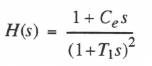
where ![]() is the rate constant and both time lags are equal to
is the rate constant and both time lags are equal to ![]() . Letting
. Letting ![]() , we can write the state equations as follows:
, we can write the state equations as follows:
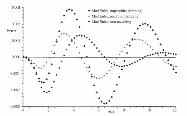
Figure 7.6. Step response errors for modified-Euler integration with and without root matching; ![]()
(7.51) ![]()
(7.52) ![]()
Eq. (7.51) represents a second-order system with an undamped natural frequency of ![]() and a damping ratio
and a damping ratio ![]() . It can be simulated with any of the modified Euler methods considered thus far in this chapter. For example, if we employ modified Euler integration with root matching, the difference equations take the form
. It can be simulated with any of the modified Euler methods considered thus far in this chapter. For example, if we employ modified Euler integration with root matching, the difference equations take the form
(7.53) ![]()
The constants D and E are given by Eqs. (7.45) and (7.46) with ![]() . In this case they can be rewritten as
. In this case they can be rewritten as
(7.54) 
To implement the output equation (7.52) we must add ![]() times the output derivative X2 to the output X1 of the second-order system. In the modified Euler method this presents a problem, since X1 is computed at integer frame times, kh, and X2 is computed at half-integer frame times, (k-1/2)h. One method for accomplishing this is to compute the output X at half-integer frame times, with
times the output derivative X2 to the output X1 of the second-order system. In the modified Euler method this presents a problem, since X1 is computed at integer frame times, kh, and X2 is computed at half-integer frame times, (k-1/2)h. One method for accomplishing this is to compute the output X at half-integer frame times, with ![]() given by the average of
given by the average of ![]() and
and ![]() . Thus the equation for the output becomes
. Thus the equation for the output becomes
(7.56) ![]()
The accuracy of the approximation ![]() can be obtained in the frequency domain by taking the Z transform of the formula using a step size of h/2 and setting
can be obtained in the frequency domain by taking the Z transform of the formula using a step size of h/2 and setting ![]() . In this way we obtain
. In this way we obtain
(7.56) 
Clearly the averaging process results in a gain error of ![]() and no phase error. When this gain error is added to the gain error of
and no phase error. When this gain error is added to the gain error of ![]() obtained earlier in Eq. (7.49), the total fractional gain error in the transfer function relating the output
obtained earlier in Eq. (7.49), the total fractional gain error in the transfer function relating the output ![]() to the input
to the input ![]() when using modified Euler with root matching is given approximately by
when using modified Euler with root matching is given approximately by ![]() . The approximate phase error remains equal to the value given in Eq. (7.49), namely
. The approximate phase error remains equal to the value given in Eq. (7.49), namely ![]() for
for ![]() .
.
In Eq. (7.52) we must also be concerned with the error in the transfer function relating the output velocity ![]() to the input
to the input ![]() . We have already determined the formula for the transfer function of the modified Euler algorithm used to integrate X2 to obtain Xl. Thus from Eq. (7.5)
. We have already determined the formula for the transfer function of the modified Euler algorithm used to integrate X2 to obtain Xl. Thus from Eq. (7.5)
(7.57) 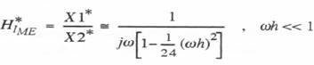
Then we can write the following formula for the transfer function ![]() relating the output X2 to the
relating the output X2 to the
input f:
(7.58) 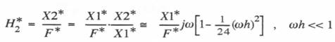
From Eq. (7.58) it is clear that the fractional gain error of ![]() is equal to the fractional gain error of the transfer function X1*/F*, i.e.,
is equal to the fractional gain error of the transfer function X1*/F*, i.e., ![]() in Eq. (7.49), plus the gain error
in Eq. (7.49), plus the gain error ![]() evident in Eq. (7.58) for the transfer function X2*/X1*. It follows that the total fractional gain error in the transfer function H2relating the velocity output X2 to the input f is given approximately by
evident in Eq. (7.58) for the transfer function X2*/X1*. It follows that the total fractional gain error in the transfer function H2relating the velocity output X2 to the input f is given approximately by ![]() . From Eq. (7.49) the approximate phase error is still given by
. From Eq. (7.49) the approximate phase error is still given by ![]() .
.
If we designate H1 as the transfer function relating X1 to f, we can then write the following formula for H*, the transfer function of the digital simulation of the controller:
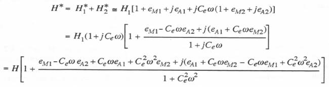
It then follows that the transfer function gain and phase errors in simulating the controller are given, respectively, by
(7.59) 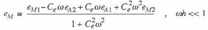
(7.60) 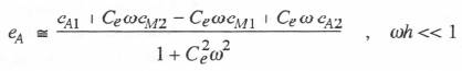
We have seen above for the modified Euler method with root matching that ![]()
![]() . Eqs. (7.59) and (7.60) can of course be used for other methods of simulating the controller, where the fractional gain errors
. Eqs. (7.59) and (7.60) can of course be used for other methods of simulating the controller, where the fractional gain errors ![]() and
and ![]() , and the phase errors
, and the phase errors ![]() and
and ![]() represent the respective gain and phase errors associated with the transfer functions relating X1 and X2 to the controller input f when using these other methods.
represent the respective gain and phase errors associated with the transfer functions relating X1 and X2 to the controller input f when using these other methods.
We now consider the time-domain errors when the various modified Euler schemes are used to simulate the linear controller. As a specific example we let ![]() , which is the same case studied in Chapter 6. We let the input be the acceleration-limited step defined in Eq. (3.176) and utilized earlier in Section 6.10. Figure 7.7 shows the controller response when the time constant of the acceleration-limited step is set equal to
, which is the same case studied in Chapter 6. We let the input be the acceleration-limited step defined in Eq. (3.176) and utilized earlier in Section 6.10. Figure 7.7 shows the controller response when the time constant of the acceleration-limited step is set equal to ![]() . Comparison with Figure 6.3 for the controller response to an ideal unit-step input confirms that the acceleration-limited step response is almost identical. As before, the rationale behind using the acceleration-limited step input is to avoid discontinuities in input displacement or velocity. Figure 7.8 shows the output error using the various modified Euler methods with an integration step size
. Comparison with Figure 6.3 for the controller response to an ideal unit-step input confirms that the acceleration-limited step response is almost identical. As before, the rationale behind using the acceleration-limited step input is to avoid discontinuities in input displacement or velocity. Figure 7.8 shows the output error using the various modified Euler methods with an integration step size ![]() . Here it would appear that the root matching technique enjoys no particular advantage over the use of predictor integration for
. Here it would appear that the root matching technique enjoys no particular advantage over the use of predictor integration for ![]() in the damping term. This is
in the damping term. This is
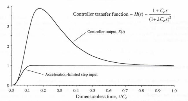
Figure 7.7. Controller response to an acceleration-limited step input.
probably because the transient is well damped ![]() and a small mismatch in transient frequency has little effect on the error.
and a small mismatch in transient frequency has little effect on the error.
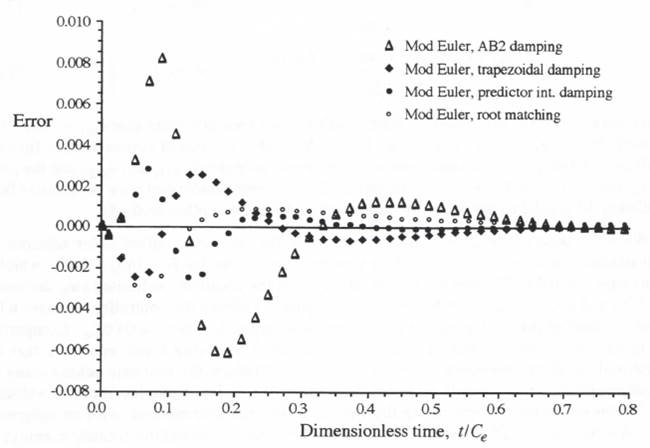
Figure 7.8. Errors in controller step response when simulated with various modified-Euler methods; step size ![]() .
.
It should be noted that Eq. (7.46) was used for the constant E in the modified Euler difference equation (7.44) for root matching when simulating an underdamped second-order system ![]() . Eq. (7.54) was used for the critically-damped case, where Eq. (7.54) follows directly from Eq. (7.46) when
. Eq. (7.54) was used for the critically-damped case, where Eq. (7.54) follows directly from Eq. (7.46) when ![]() . For the overdamped case
. For the overdamped case ![]() we can still use Eq. (7.46) if we note that
we can still use Eq. (7.46) if we note that ![]() . Thus for
. Thus for ![]() Eq. (7.46) becomes
Eq. (7.46) becomes
(7.61) ![]()
In either Eq. (7.44) or Eq. (7.53) the constant D given by Eq. (7.45) applies for all ![]() .
.
7.9 Comparison of Modified Euler and State-transition Methods
It is instructive to compare the results we have obtained above using modified Euler simulation of the controller with the results obtained when the state-transition method introduced in Chapter 6 is used. This comparison is especially appropriate when modified Euler with root-matching is used, since both methods then match the characteristic roots of the linear system being simulated. In Chapter 6 we observed that the only error exhibited by the state transition method is that associated with the formula used to approximate the input f(t) in the definite-integral portion of the state-transition difference equation. In Table 6.1 we summarized the transfer function gain and phase errors for a number of candidate methods for this approximation. One method not considered in Chapter 6 involves letting the input approximation ![]() , i.e., the input represented halfway through the frame. This is a particularly good choice in comparing results with the modified Euler scheme, because both methods then compute the controller output data point one-half frame time after the input data point.
, i.e., the input represented halfway through the frame. This is a particularly good choice in comparing results with the modified Euler scheme, because both methods then compute the controller output data point one-half frame time after the input data point.
When the state-transition method is used to simulate the controller equations (7.51) and (7.52) with ![]() , the following difference equations result:
, the following difference equations result:
(7.62) ![]()
(7.63) ![]()
Here the coefficients w11, w12, w21 and w22 are given by Eq. (6.73). The formulas for b1 and b2 are
(7.64) ![]()
where U(t) and ![]() are given in Eqs. (6.74) and (6.75) and represent, respectively, the unit step response and unit impulse response of the second-order system.
are given in Eqs. (6.74) and (6.75) and represent, respectively, the unit step response and unit impulse response of the second-order system.
For an integration step size h = 0.02Ce, Figure 7.9 shows the output errors when the controller
Figure 7.9. Errors in controller step response when simulated using the state-transition method and various modified-Euler methods.
is simulated by the above state-transition method, as well as the three different modified-Euler methods. All the methods appear to give comparable results, although the state-transition method exhibits the largest startup transient error. Subsequently, however, the state-transition error damps more quickly to zero. The modified-Euler method which uses predictor integration for the integer-frame estimate of X2 seems to give the best overall results and it is equally applicable to nonlinears systems. As noted in Figure 7.2, it does have a more restricted stability region in the ![]() plane.
plane.
In addition to comparing the time-domain performance of the state-transition method with the various modified-Euler schemes, it is useful to compare the frequency-domain performance. For the state-transition method considered here, where we represent f (t) in the definite integral by ![]() , it is simpler to determine first the transfer function when simulating the first-order system with characteristic root
, it is simpler to determine first the transfer function when simulating the first-order system with characteristic root ![]() , i.e., the system given by Eq. (6.4) with
, i.e., the system given by Eq. (6.4) with ![]() . From Eq. (6.14) with
. From Eq. (6.14) with ![]() , replaced by
, replaced by ![]() , we have the following difference equation:
, we have the following difference equation:
(7.65) 
Taking the Z transform with a step size of h/2 and setting ![]() , we obtain the transfer function for sinusoidal inputs, from which the following approximate formulas for the fractional gain error and phase error can be derived:
, we obtain the transfer function for sinusoidal inputs, from which the following approximate formulas for the fractional gain error and phase error can be derived:
(7.66) 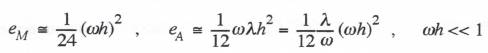
Comparison with the transfer function errors in Table 6.1 shows that the above gain error is smaller than the gain error for any of the second-order methods in the table. However, there is a finite phase error in Eq. (7.66), as opposed to zero phase error to order h2 for the second-order methods in Table 6.1. Furhermore, the phase error in Eq. (7.66) depends on the eigenvalue ![]() ., which means that the approximate transfer function error when using the state-transition method with
., which means that the approximate transfer function error when using the state-transition method with ![]() does depend on the system being simulated and not simply
does depend on the system being simulated and not simply ![]() .
.
The above results for simulating a first -order system can be extended to a second-order system with characteristic roots ![]() and
and ![]() and transfer function H(s) by noting that
and transfer function H(s) by noting that
(7.67)
In terms of the fractional gain error ![]() and the phase error
and the phase error ![]() associated with the digital transfer function H* in simulating a continuous system with transfer function
associated with the digital transfer function H* in simulating a continuous system with transfer function ![]() , we recall that
, we recall that ![]() . From Eqs. (7.66) and (7.67) it follows that
. From Eqs. (7.66) and (7.67) it follows that
or
Thus the transfer function fractional gain error and phase error, respectively, when the state transition
method based on ![]() is used to simulate a second-order linear system, are given by
is used to simulate a second-order linear system, are given by
(7.68) ![]()
Unlike the first-order system simulation, which in Eq. (7.66) exhibits a,phase error as well as a gain error of order h2, here the second-order system simulation based on ![]() in the state-transition formulation only exhibits a gain error, an error which is independent of the system parameters and depends only on
in the state-transition formulation only exhibits a gain error, an error which is independent of the system parameters and depends only on ![]()
The results in Eq. (7.66) for the gain and phase errors in state-transition simulation of a first order system can also be extended to a second-order system when the output is considered to be the time-derivative state, X2. Thus we note that
(7.69) 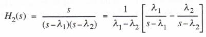
Again using the formulas in Eq. (7.66) for the fractional gain and phase errors in simulating the first-order systems in Eq. (7.69), we can derive, the equations for the approximate gain and phase errors when the state-transition method with ![]() is used to simulate the second-order system represented by Eq. (7.69). In this way we obtain
is used to simulate the second-order system represented by Eq. (7.69). In this way we obtain
(7.70) 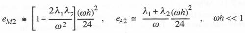
From Eq. (7.14) we note that ![]() and
and ![]() . With these substitutions we can rewrite Eq. (7.70) as
. With these substitutions we can rewrite Eq. (7.70) as
(7.71) 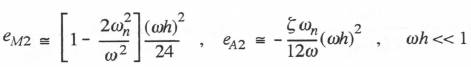
Substituting ![]() and
and ![]() from Eq. (7.68) and
from Eq. (7.68) and ![]() and
and ![]() from Eq. (7.71) into Eq. (7.59) and (7.60), we can write the formulas for the approximate gain and phase errors when the state-transition method with
from Eq. (7.71) into Eq. (7.59) and (7.60), we can write the formulas for the approximate gain and phase errors when the state-transition method with ![]() is used to simulate the second-order controller.
is used to simulate the second-order controller.
The gain and phase errors in Eq. (7.71) for the state-transition method with ![]() when simulating the second-order system of Eq. (7.69) should be compared with the errors when modified Euler simulation with root matching is used. Adding the gain error of
when simulating the second-order system of Eq. (7.69) should be compared with the errors when modified Euler simulation with root matching is used. Adding the gain error of ![]() in Eq. (7.58) to the gain and phase errors in Eq. (7.49), we obtain
in Eq. (7.58) to the gain and phase errors in Eq. (7.49), we obtain
(7.72) 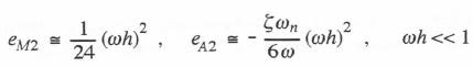
Comparison of the results in Eq. (7.71) for the state-transition method based on ![]() with the above results in Eq. (7.72) for the modified-Euler method with root matching shows that the phase error in the output derivative X2 in the case of the state-transition method is half as large. On the other hand, for very low input frequencies, i.e.,
with the above results in Eq. (7.72) for the modified-Euler method with root matching shows that the phase error in the output derivative X2 in the case of the state-transition method is half as large. On the other hand, for very low input frequencies, i.e., ![]() , comparison of Eq. (7.71) with Eq. (7.72) shows that the magnitude of the gain error
, comparison of Eq. (7.71) with Eq. (7.72) shows that the magnitude of the gain error ![]() for the state-transition method is much larger than the magnitude of
for the state-transition method is much larger than the magnitude of ![]() for the modified-Euler method, namely
for the modified-Euler method, namely ![]() times larger. For very high input frequencies, i.e.,
times larger. For very high input frequencies, i.e., ![]() , comparison of Eq. (7.71) with (7.72) shows that the gain errors in the output derivative X2 are equal for the two methods. When the output of the second-order system is the displacement state X1 rather than the velocity state X2, we have seen that the state-transition gain error in Eq. (7.68) is half the magnitude of the modified Euler gain error in Eq. (7.49). Also, the state-transition phase error in Eq. (7.68) is zero to order h2, compared with the finite modified-Euler phase error of order h2 in Eq. (7.49). However, the output displacement when using the modified-Euler method is
, comparison of Eq. (7.71) with (7.72) shows that the gain errors in the output derivative X2 are equal for the two methods. When the output of the second-order system is the displacement state X1 rather than the velocity state X2, we have seen that the state-transition gain error in Eq. (7.68) is half the magnitude of the modified Euler gain error in Eq. (7.49). Also, the state-transition phase error in Eq. (7.68) is zero to order h2, compared with the finite modified-Euler phase error of order h2 in Eq. (7.49). However, the output displacement when using the modified-Euler method is ![]() for an input
for an input ![]() , as is apparent in Eq. (7.53). For the state-transition method Eq. (7.62) shows that the output is
, as is apparent in Eq. (7.53). For the state-transition method Eq. (7.62) shows that the output is ![]() for an input
for an input ![]() . Thus the modified-Euler output displacement leads the state-transition output by half a time step for the same input data sequence in simulating a second-order system. This can represent a significant advantage in many applications. We conclude that relative to each other, the modified -Euler method with root-matching and the state-transition method have both advantages and disadvantages, with the optimal choice dependent upon the particular requirements in any given simulation application.
. Thus the modified-Euler output displacement leads the state-transition output by half a time step for the same input data sequence in simulating a second-order system. This can represent a significant advantage in many applications. We conclude that relative to each other, the modified -Euler method with root-matching and the state-transition method have both advantages and disadvantages, with the optimal choice dependent upon the particular requirements in any given simulation application.
7.10 Simulation of a Fourth-order Bandpass Filter
The modified Euler method with root matching becomes especially effective in simulating high-order linear systems, such as those used to represent linear filters.* We next consider a fourth-order linear system consisting of two velocity-output second-order systems in series, as shown in Figure 7.10. When the second-order systems are lightly-damped, each with a slightly different undamped natural frequency and damping ratio, the fourth-order system can be used to synthesize a narrow-bandpass filter. Thus we let the filter transfer function be given by
(7.73) ![]()
where
(7.74) 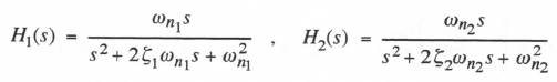
We simulate each of the second-order systems with the root-matching version of modified Euler integration that uses Eqs. (7.44), (7.45) and (7.46). With ![]() as the input to the first subsystem, we recall from the previous section that the output after completion of the integration step is equal to
as the input to the first subsystem, we recall from the previous section that the output after completion of the integration step is equal to ![]() , with the transfer function gain and phase errors given by Eq. (7.72). If
, with the transfer function gain and phase errors given by Eq. (7.72). If ![]() is then used as the input to the second subsystem, the output will be
is then used as the input to the second subsystem, the output will be ![]() , as indicated in Figure 7.10. The approximate overall transfer function gain and phase errors to order h2 will then be the sum of the individual subsystem gain and phase errors of Eq. (7.72). Thus
, as indicated in Figure 7.10. The approximate overall transfer function gain and phase errors to order h2 will then be the sum of the individual subsystem gain and phase errors of Eq. (7.72). Thus
* See, for example, Howe, R.M., “Simulation of Linear Systems Using Modified Euler Integration Methods,” Transactions of the Society for Computer Simulation, Vol. 5, No. 2, 1985, pp 125-152.
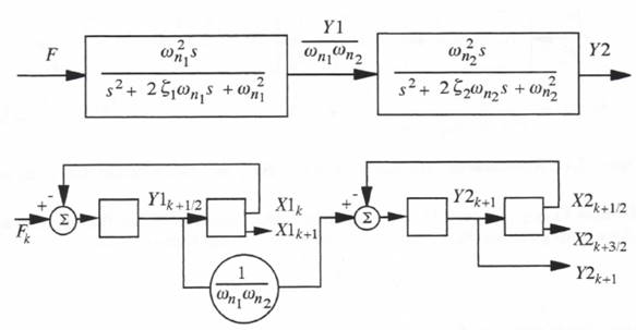
Figure 7.10. Fourth-order bandpass filter synthesized with two modified-Euler subsystems.
(7.75) 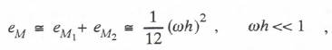
(7.76) 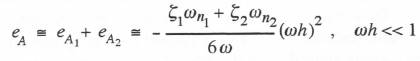
The extension to any linear system that can be represented by second-order subsystems in series is obvious. To order h2 the asymptotic formulas for transfer function gain and phase errors are given simply by the sum of the gain and phase errors for each of the individual subsystems. If the second-order subsystems have velocity instead of displacement as outputs, then each output represents a half-integer sample with respect to the input, as shown in Figure 7.10. Under these conditions an odd number of second-order subsystems will lead to a half-integer output sample. If an integer output sample is required, it can be computed as the average of the two half-integer samples bracketing the integer sample point.
7.11 Modified Euler Simulation of a 14th-order Bandpass Filter
In this section we consider a 14th-order bandpass filter. The filter is synthesized with 3 pairs of second-order filters plus a single second-order filter, all connected in series as shown in Figure 7.11. Each pair of second-order filters represents a fourth-order filter with the transfer function defined as in Eqs. (7.73) and (7.74). Each individual second-order subsystem is simulated using the modified Euler algorithm with root matching, as given earlier in Eqs. (7.44), (7.45) and (7.46). Within each pair of second-order systems the updated velocity of the first subsystem, designated ![]() in Figure 7.10, is used to provide the input to the second sub-system. For the subsystem
in Figure 7.10, is used to provide the input to the second sub-system. For the subsystem ![]() in Figure 7.11 the output
in Figure 7.11 the output ![]() rather than the updated output
rather than the updated output ![]() is used as the input for the second subsystem,
is used as the input for the second subsystem, ![]() . The output
. The output ![]() instead of the updated output
instead of the updated output ![]() of this second subsystem is in turn used as the input to the third subsystem,
of this second subsystem is in turn used as the input to the third subsystem, ![]() . Here the updated output
. Here the updated output ![]() drives the final second order subsystem
drives the final second order subsystem ![]() , which then produces the updated
, which then produces the updated
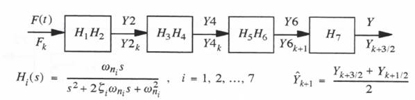
Figure 7.11. Synthesis of 14th-order bandpass filter as 7 second-order filters in series.
output ![]() . To provide the overall filter output estimate
. To provide the overall filter output estimate ![]() at the integer frame time
at the integer frame time ![]() we simply average
we simply average ![]() and
and ![]() (from the previous frame). Thus
(from the previous frame). Thus
(7.77) 
We have already seen from Eq. (7.56) that the transfer function represented by the averager of Eq. (7.77) exhibits zero phase error and has a gain error given approximately by ![]() .
.
We are now in a position to estimate the overall transfer function gain and phase errors in simulating the 14th-order filter. Eqs. (7.75) and (7.76) give the gain and phase errors for each of the three pairs of second-order systems. Eq. (7.72) gives the gain and phase error for the single second-order system. Finally, Eq. (7.56) gives the gain error in the calculation of ![]() at the integer frame time
at the integer frame time ![]() from
from ![]() and
and ![]() . As noted earlier, to order
. As noted earlier, to order ![]() the overall gain and phase errors are the sum, respectively, of the individual gain and phase errors. In this way we obtain the following asymptotic formulas for the overall gain and phase errors for our modified Euler simulation of the 14th-order bandpass filter.
the overall gain and phase errors are the sum, respectively, of the individual gain and phase errors. In this way we obtain the following asymptotic formulas for the overall gain and phase errors for our modified Euler simulation of the 14th-order bandpass filter.
(7.78) 
As a specific example we consider the 14th-order Chebychev bandpass filter with the undamped natural frequencies and damping ratios given in Table 7.5 for the individual second-order systems. The frequencies have been normalized so that the center frequency of the overall filter is unity. Figure (7.12) shows the frequency response of the filter.
Table 7.5
Undamped Natural Frequencies and Damping Ratios for Second-order Subsystems in a 14th-order Chebychev Bandpass Filter
From Eq. (7.78) it is apparent that the gain error in simulating the filter is independent of the filter parameters and depends only on ![]() , i.e., the input frequency times the step size. If we substitute the damping ratio values of Table 7.5 into Eq. (7.79), the resulting phase shift error becomes
, i.e., the input frequency times the step size. If we substitute the damping ratio values of Table 7.5 into Eq. (7.79), the resulting phase shift error becomes
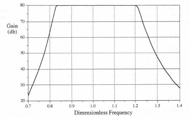
Figure 7.12. Frequency response of 14th-order Chebychev bandpass filter.
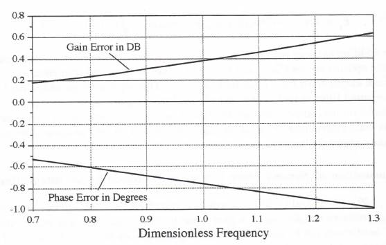
Figure 7.13. Gain and phase errors for modified-Euler simulation of 14th-order Chebychev bandpass filter. Integration step size h = 0.5.
![]() . For input frequencies
. For input frequencies ![]() this corresponds to a phase error of approximately
this corresponds to a phase error of approximately ![]() radians. The gain error from Eq. (7.79) for
radians. The gain error from Eq. (7.79) for ![]() is approximately
is approximately ![]() . As a specific example, consider a step-size
. As a specific example, consider a step-size ![]() , which corresponds to 2 integration steps per radian or 12.57 steps per cycle of the center bandpass frequency of the filter. For this relative-ly large integration step the plots in Figure 7.13 show that the average gain error is about 0.4 db and the average phase error is about – 0.7 degrees over the bandpass of the filter.
, which corresponds to 2 integration steps per radian or 12.57 steps per cycle of the center bandpass frequency of the filter. For this relative-ly large integration step the plots in Figure 7.13 show that the average gain error is about 0.4 db and the average phase error is about – 0.7 degrees over the bandpass of the filter.
The actual difference equations which are solved each integration step are summarized below, where half-integer indices are used when the state variables are interpreted as representing half-integer samples.
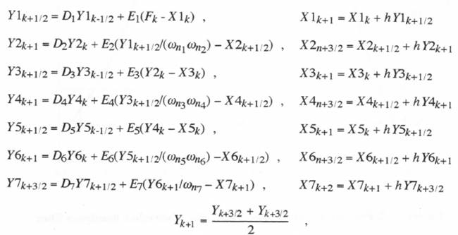
(7.79)
where

(7.80)
If, in addition to using the updated value, ![]() , to drive the seventh equation in (7.80), we also use the updated values
, to drive the seventh equation in (7.80), we also use the updated values ![]() and
and ![]() to drive the third and fifth equations, respectively, then the final output from Eq. (7.80) will be
to drive the third and fifth equations, respectively, then the final output from Eq. (7.80) will be ![]() . This represents an additional lead time of 2h in the computed filter output at the end of the kth integration frame. This lead could be potentially useful for the compensation of interface delays in a real-time simulation. Our algorithm in this case is taking advantage of the basic lags associated with the bandpass filter to produce a lead time in the computed filter response.
. This represents an additional lead time of 2h in the computed filter output at the end of the kth integration frame. This lead could be potentially useful for the compensation of interface delays in a real-time simulation. Our algorithm in this case is taking advantage of the basic lags associated with the bandpass filter to produce a lead time in the computed filter response.
7.12 Compensation of Second-order Errors in Modified Euler Integration
Eqs. (7.49), (7.72) and (7.78) all show that modified Euler integration, when used with root matching, produces transfer-function gain errors proportional to ![]() and phase errors proportional to
and phase errors proportional to ![]() . These errors can be cancelled by adding appropriate terms to the output of the digital simulation. For example, consider an output term
. These errors can be cancelled by adding appropriate terms to the output of the digital simulation. For example, consider an output term ![]() given by the equation
given by the equation
(7.81) ![]()
where the velocity state variable Y is related to the displacement state variable X by Eq. (7.8). Thus
(7.82) 
Then Eq. (7.81) can be rewritten in terms of ![]() with the following formula:
with the following formula:
(7.83) 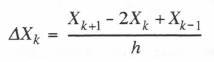
Here we recognize that ![]() is proportional to the central difference approximation for the second time derivative of X. Taking the Z transform of Eq. (7.83) and solving for the transfer function which relates
is proportional to the central difference approximation for the second time derivative of X. Taking the Z transform of Eq. (7.83) and solving for the transfer function which relates ![]() to X*, we obtain
to X*, we obtain
(7.84) 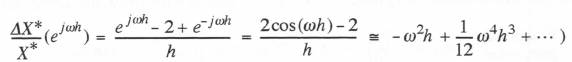
Here ![]() represents a transfer function proportional to
represents a transfer function proportional to ![]() for
for ![]() . This is not surprising, since
. This is not surprising, since ![]() is proportional to the second time derivative of X which, for sinusoidal inputs, is in turn proportional to
is proportional to the second time derivative of X which, for sinusoidal inputs, is in turn proportional to ![]() .
.
We next consider an output term ![]() given by the equation
given by the equation
(7.85) ![]()
Taking the Z transform and solving for the transfer function that relates ![]() to
to ![]() , we obtain
, we obtain
(7.86) 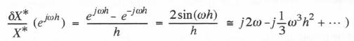
Here ![]() represents a transfer function proportional to
represents a transfer function proportional to ![]() for
for ![]() . Again this is to be expected, since
. Again this is to be expected, since ![]() in Eq. (7.85) is proportional to Y, the time derivative of X, which in turn is proportional to
in Eq. (7.85) is proportional to Y, the time derivative of X, which in turn is proportional to ![]() .
.
To illustrate the use of ![]() and
and ![]() , as defined above, to cancel the modified-Euler transfer function errors of order h2, we consider the case of modified Euler integration with root matching applied to a second-order linear system. From Eq. (7.49) the asymptotic formula for the transfer function ratio is given by
, as defined above, to cancel the modified-Euler transfer function errors of order h2, we consider the case of modified Euler integration with root matching applied to a second-order linear system. From Eq. (7.49) the asymptotic formula for the transfer function ratio is given by
(7.87) 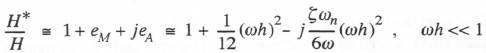
We now define a new output variable ![]() given by
given by
(7.88) 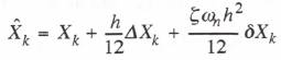
Taking the Z transform of Eq. (7.88) and solving for ![]() , we obtain from Eqs. (7.84) and (7.86) the following asymptotic formula:
, we obtain from Eqs. (7.84) and (7.86) the following asymptotic formula:
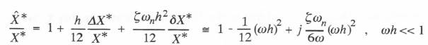
(7.89)
The transfer function ratio ![]() for the new output
for the new output ![]() is given by the product of Eqs. (7.87) and (7.89). Thus
is given by the product of Eqs. (7.87) and (7.89). Thus
(7.90) 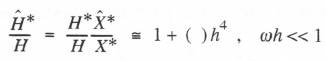
Here the transfer function gain and phase errors of order ![]() result from the terms of order
result from the terms of order ![]() which were neglected in Eqs. (7.49) for
which were neglected in Eqs. (7.49) for ![]() and
and ![]() as well as the terms of order
as well as the terms of order ![]() when Eqs. (7.84) and (7.86) are substituted into Eq. (7.89). When the terms of order
when Eqs. (7.84) and (7.86) are substituted into Eq. (7.89). When the terms of order ![]() are taken into account, we obtain the following formulas for the gain and phase errors in the transfer function
are taken into account, we obtain the following formulas for the gain and phase errors in the transfer function ![]() for the second-order system simulated using modified-Euler integration with quadratic compensation:
for the second-order system simulated using modified-Euler integration with quadratic compensation:
(7.91) 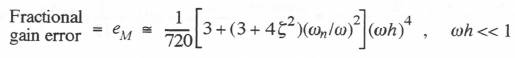
(7.92) 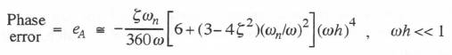
For ![]() Figure 7.14 shows plots of the exact gain and phase error versus frequency for
Figure 7.14 shows plots of the exact gain and phase error versus frequency for ![]() and 1.0. The results, even for
and 1.0. The results, even for ![]() , agree quite closely with the approximate errors given above in Eqs. (7.91) and (7.92). Note that for
, agree quite closely with the approximate errors given above in Eqs. (7.91) and (7.92). Note that for ![]() the gain and phase errors are less than those given by Eq. (7.49) for
the gain and phase errors are less than those given by Eq. (7.49) for ![]() when modified Euler integration with root matching but without quadratic compensation is used. Note also that both the gain and phase errors in Figure 7.14 are reduced by a factor of 16 when the step size is halved to
when modified Euler integration with root matching but without quadratic compensation is used. Note also that both the gain and phase errors in Figure 7.14 are reduced by a factor of 16 when the step size is halved to ![]() . This demonstrates that the quadratic compensation does indeed change the modified Euler method to a fourth-order algorithm.
. This demonstrates that the quadratic compensation does indeed change the modified Euler method to a fourth-order algorithm.
It should be noted that the use of Eq. (7.81) or (7.83) for ![]() and (7.85) for
and (7.85) for ![]() requires values
requires values ![]() or
or ![]() at the end of the kth integration frame in order to compute
at the end of the kth integration frame in order to compute ![]() at the beginning of the kth frame using Eq. (7.88). This means that the compensated output
at the beginning of the kth frame using Eq. (7.88). This means that the compensated output ![]() will be delayed with respect to real time by one integration step in the simulation of a second-order system. As we shall see in the next paragraph, the quadratic compensation scheme described here can be used to provide real-time outputs in simulating linear systems of order four or higher. Calculation of the compensated output
will be delayed with respect to real time by one integration step in the simulation of a second-order system. As we shall see in the next paragraph, the quadratic compensation scheme described here can be used to provide real-time outputs in simulating linear systems of order four or higher. Calculation of the compensated output ![]() using Eqs. (7.81), (7.85) and (7.88) only requires two more multiplications and four more additions each integration frame, since the coefficients of
using Eqs. (7.81), (7.85) and (7.88) only requires two more multiplications and four more additions each integration frame, since the coefficients of ![]() and
and ![]() in Eq. (7.88) are fixed constants that can be precomputed.
in Eq. (7.88) are fixed constants that can be precomputed.
We consider next the use of quadratic compensation in the modified Euler simulation of the 14th-order bandpass filter described in Section 7.11. The gain and phase errors of order ![]() for the transfer function are given in Eq. (7.78). Here we will use the state variable Y6 in Figure 7.11 to provide the compensation. Thus we define
for the transfer function are given in Eq. (7.78). Here we will use the state variable Y6 in Figure 7.11 to provide the compensation. Thus we define ![]() and
and ![]() with the following formulas:
with the following formulas:
(7.93) ![]()
With the procedures used earlier in deriving Eqs. (7.84) and (7.86) the following formulas are obtained
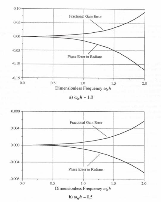
Figure 7.14. Gain and phase errors in simulating a second-order system using modified-Euler integration with quadratic compensation; ![]() .
.
for the incremental transfer functions ![]() and
and ![]() :
:
(7.94) 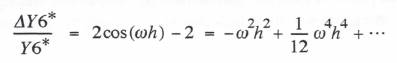
(7.95) 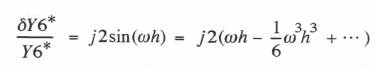
Comparison with Eq. (7.78) shows that the overall transfer function gain and phase errors of order h2 in the simulation of the bandpass filter can be cancelled by letting ![]() be the input to the last second-order subsystem in Figure 4, where
be the input to the last second-order subsystem in Figure 4, where ![]() is given by
is given by
(7.96) 
Thus ![]() in the next to last equation in (7.80) is replaced by
in the next to last equation in (7.80) is replaced by ![]() . From Eqs. (7.94) and (7.97) we see that the calculation of
. From Eqs. (7.94) and (7.97) we see that the calculation of ![]() utilizes
utilizes ![]() and
and ![]() . To obtain
. To obtain ![]() in the kth integration frame will require another one-frame advance in Eq. (7.79). This can be achieved by letting
in the kth integration frame will require another one-frame advance in Eq. (7.79). This can be achieved by letting ![]() rather than
rather than ![]() be the input to the fifth equation in (7.79). The modified-Euler simulation with quadratic compensation will now exhibit transfer-function gain and phase errors proportional to h4. For the specific bandpass filter considered earlier, Figure 7.15 shows a plot of the errors for h = 0.5. Comparison with Figure 7.13 shows that we have reduced the gain and phase errors by factors of approximately 25 and 50, respectively. Because of the dependence on h4 this means the errors will increase by a factor of 16 if we double the step size to h = 1. Even then the errors will be significantly less than those obtained earlier for h = 0.5 when quadratic compensation was not used.
be the input to the fifth equation in (7.79). The modified-Euler simulation with quadratic compensation will now exhibit transfer-function gain and phase errors proportional to h4. For the specific bandpass filter considered earlier, Figure 7.15 shows a plot of the errors for h = 0.5. Comparison with Figure 7.13 shows that we have reduced the gain and phase errors by factors of approximately 25 and 50, respectively. Because of the dependence on h4 this means the errors will increase by a factor of 16 if we double the step size to h = 1. Even then the errors will be significantly less than those obtained earlier for h = 0.5 when quadratic compensation was not used.
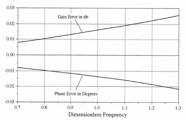
Figure 7.15. Gain and phase errors for simulation of 14th-order bandpass filter using modified-Euler integration with quadratic compensation. Step – size h = 0.5.
The quadratic compensation of Eqs. (7.93) and (7.96) adds only 3 multiplications and 5 additions to the overall computation, which now takes a total of 29 multiplications and 29 additions per integration step. This is far less than the required number of multiplications and additions for any other fourth-order method when applied to this 14th-order filter problem.
7.13 The Use of Input Averaging with Modified Euler Integration
In Chapter 5, Section 5.11, we introduced the concept of multi-rate sampling and averaging of a continuous input to a real-time simulation. It was pointed out that this procedure can be used to reduce the “aliasing” effect, i.e., the conversion of input frequencies above one-half the frame rate to frequencies below one-half the frame rate. As the number of samples N per frame approaches infinity, we observed in Eq. (5.83) that the averager transfer function, ![]() , is given by
, is given by
(7.97) 
It was also noted in Section 5.11 that the average of N input samples of f(t) over the kth frame, i.e., from ![]() to
to ![]() can be considered equivalent to a sample-data point at the midpoint of the frame, denoted by
can be considered equivalent to a sample-data point at the midpoint of the frame, denoted by ![]() . For the state equation
. For the state equation ![]() this data point can then be used as the input to the modified Euler integration algorithm
this data point can then be used as the input to the modified Euler integration algorithm
(7.98) ![]()
If the modified-Euler integrator transfer function ![]() derived earlier in Eq. (7.5) is multiplied by
derived earlier in Eq. (7.5) is multiplied by ![]() in Eq. (7.98), the resulting product,
in Eq. (7.98), the resulting product, ![]() is exactly
is exactly ![]() , the ideal integrator transfer function. This is not surprising, since the average of f(t) is obtained by integrating f(t) over the kth frame and dividing the result by h. When the average is then multiplied by h, as in Eq. (7.99), the result is indeed the exact integral of f(t) over the kth frame.
, the ideal integrator transfer function. This is not surprising, since the average of f(t) is obtained by integrating f(t) over the kth frame and dividing the result by h. When the average is then multiplied by h, as in Eq. (7.99), the result is indeed the exact integral of f(t) over the kth frame.
It is useful to examine the accuracy improvement which results when input averaging is utilized in an actual simulation. For example, consider again the second order system given by Eq. (7.6) when subjected to the acceleration-limited step input U(t) of Eq. (7.29). When input averaging is applied to U(t), the resulting errors in simulated output using various modified Euler methods are shown in Figure 7.16. Comparison with the previous results without input averaging, as shown earlier in Figure 7.6, demonstrates that the use of input averaging has indeed reduced the output error. Of course, it has not eliminated the error, since the ideal integrator behavior associated with input averaging applies only to the input term U(t) on the right side of the equation for ![]() in (7.6). As noted above, however, the input averaging will reduce significantly the errors caused by sampling any frequencies above one-half the frame rate 1/h which may be present in U(t).
in (7.6). As noted above, however, the input averaging will reduce significantly the errors caused by sampling any frequencies above one-half the frame rate 1/h which may be present in U(t).
The accuracy improvement obtained using input averaging becomes much greater in the case of inputs with discontinuities. To illustrate this, we consider a simulation of the unit step response of a Butterworth low-pass filter.* The transfer function gain of a Butterworth filter of order
* Oppenheim, A.V., and R.V. Schafer, Digital Signal Processing, Prentiss-Hall, Englewood Cliffs, New Jersey, 1975.
7-35
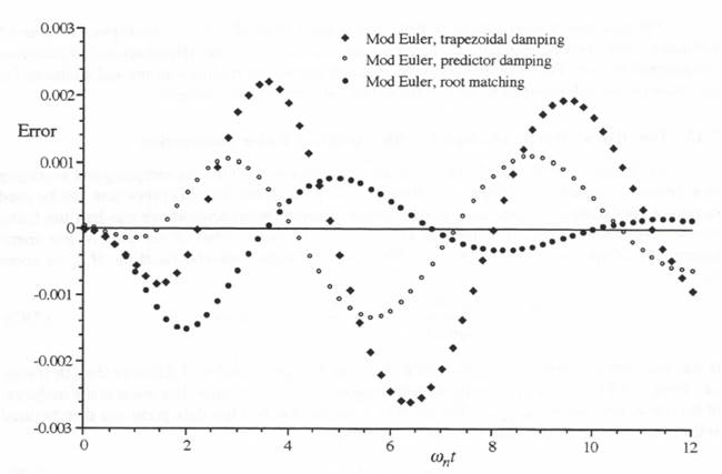
Figure 7.16. Acceleration-limited step response errors for modified-Euler methods when using input averaging; ![]() .
.
n with a cutoff frequency of ![]() is given by the formula
is given by the formula
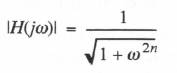
(7.99)
The gain characteristic exhibited by Eq. (7.99) represents the sharpest cutoff achievable by a low-pass filter of order n without any rise in filter gain above its zero-frequency value of unity. For a 6th-order Butterworth filter (n = 6) Figure 7.17 shows the transfer function gain ![]() versus frequency
versus frequency ![]() .
.
It can be shown that the n characteristic roots of the Butterworth filter are distributed with equal polar angle separation on the unit half-circle in the left s plane. For example, if n = 6, the characteristic roots (i.e., transfer function poles) are given by ![]() ,
, ![]() and
and ![]() . The corresponding damping ratios of the three root pairs are equal to
. The corresponding damping ratios of the three root pairs are equal to ![]() ,
, ![]() and
and ![]() . Thus
. Thus
![]()
The transfer function of the 6th-order filter is then given by
Figure 7.17. Frequency response of 6t-order Butterworth filter.
(7.100) 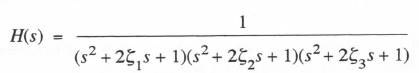
Each of the three second-order transfer functions represented in Eq. (7.100) can be simulated using the modified-Euler method with root matching, as given by Eq. (7.44), This results in the following difference equations:
(7.101) 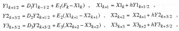
where the coefficients D and E are given by Eqs. (7.45) and (7.46). Note in (7.101) that we have used the updated output of the first 2nd-order subsystem, ![]() , as the input to the second subsystem, and the updated output of the second subsystem,
, as the input to the second subsystem, and the updated output of the second subsystem, ![]() , as the input to the third subsystem. In this way the final filter output, X = X3, at the end of the kth integration frame, is actually
, as the input to the third subsystem. In this way the final filter output, X = X3, at the end of the kth integration frame, is actually ![]() rather than
rather than ![]() . In a real-time simulation this means that the output is available two frames ahead of its occurrence in real time. On the other hand, when we replace the input
. In a real-time simulation this means that the output is available two frames ahead of its occurrence in real time. On the other hand, when we replace the input ![]() by
by ![]() , its average over the interval from
, its average over the interval from ![]() to
to ![]() , we cannot begin the computation for the kth frame until
, we cannot begin the computation for the kth frame until ![]() . In this case the output
. In this case the output ![]() will become available at
will become available at ![]() , not
, not ![]() . Furthermore, if we apply the quadratic compensation described in Section 7.12 using central-difference formulas, we will need the outputs one frame ahead of when they would occur in real time in order to produce a compensated real-time output. Thus input averaging and quadratic compensation will use up one and a half frames of the two-frame lead we have realized in the mechanization of Eq. (7.101).
. Furthermore, if we apply the quadratic compensation described in Section 7.12 using central-difference formulas, we will need the outputs one frame ahead of when they would occur in real time in order to produce a compensated real-time output. Thus input averaging and quadratic compensation will use up one and a half frames of the two-frame lead we have realized in the mechanization of Eq. (7.101).
When using the modified Euler method with root matching, Eq. (7.49) gives the approximate transfer function gain and phases errors for each of the second-order subsystem simulations. It follows that the approximate gain and phase errors for the overall simulation will simply be the sum of the individual errors. Thus
(7.102) 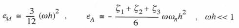
where ![]() in our example here. To cancel these second-order terms we use Eqs. (7.81) and (7.85) for
in our example here. To cancel these second-order terms we use Eqs. (7.81) and (7.85) for ![]() and
and ![]() , with
, with ![]() and
and ![]() replaced by
replaced by ![]() and
and ![]() , respectively. From Eqs. (7.84) and (7.86) it then becomes apparent that the compensated output variable,
, respectively. From Eqs. (7.84) and (7.86) it then becomes apparent that the compensated output variable, ![]() , is given by the formula
, is given by the formula
(7.103) 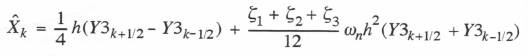
with ![]() again equal to 1 on our example. We note that Eq. (7.103) can be rewritten as
again equal to 1 on our example. We note that Eq. (7.103) can be rewritten as
(7.104) 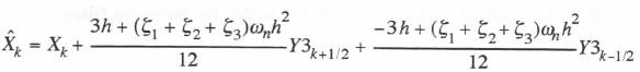
Since the coefficients of ![]() and
and ![]() can be precomputed, it is apparent that the quadratic compensation only requires 2 multiplies and 2 adds per integration frame.
can be precomputed, it is apparent that the quadratic compensation only requires 2 multiplies and 2 adds per integration frame.
The quadratic compensation given by Eq. (7.104) is based on using the direct input data point ![]() for the kth integration frame in Eq. (7.101). If we use the input averaging described in Section 5.11, where we replace
for the kth integration frame in Eq. (7.101). If we use the input averaging described in Section 5.11, where we replace ![]() by its average over the time frame centered about kh, namely,
by its average over the time frame centered about kh, namely, ![]() , Eq. (7.97) shows that an additional gain error equal to
, Eq. (7.97) shows that an additional gain error equal to ![]() will be introduced for
will be introduced for ![]() . When this is added to the gain error of
. When this is added to the gain error of ![]() in Eq. (7.102), the overall gain error in simulating the filter becomes approximately
in Eq. (7.102), the overall gain error in simulating the filter becomes approximately ![]() . Under these conditions the quadratic compensation formula of Eq. (7.104), when input averaging is also used, becomes
. Under these conditions the quadratic compensation formula of Eq. (7.104), when input averaging is also used, becomes
(7.105) 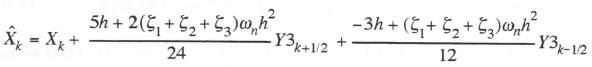
We now consider simulation of the 6th-order Butterworth filter response to a unit step input using Modified Euler integration with root matching. In Figure 7.18 the exact response to an ideal step input occurring at t = 0 is shown. Figure 7.19 shows the simulation error with and without quadratic compensation. In both cases the integration step size h = 0.2 and input averaging is employed, i.e., ![]() in Eq. (7.101) is replaced by
in Eq. (7.101) is replaced by ![]() For the unit step input at t = 0 this means that
For the unit step input at t = 0 this means that ![]() is equal to 0.5, the average value of the input from –h/2 to h/2. The input
is equal to 0.5, the average value of the input from –h/2 to h/2. The input ![]() for subsequent frames, where
for subsequent frames, where ![]() is equal to 1. When quadratic compensation is used in accordance with Eq. (7.106) to calculate the final filter output
is equal to 1. When quadratic compensation is used in accordance with Eq. (7.106) to calculate the final filter output ![]() , it is apparent in Figure 7.19 that the simulation error is reduced very substantially.
, it is apparent in Figure 7.19 that the simulation error is reduced very substantially.
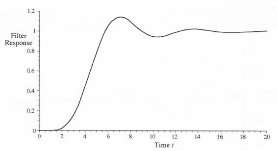
Figure 7.18. Exact 6th-order Butterworth filter response to a unit-step input.
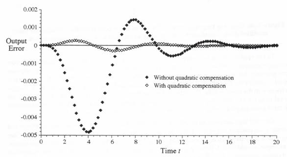
Figure 7.19. Unit step response errors of 6th-order Butterworth filter simulation using modified-Euler integration with root matching, input averaging; h = 0.2
.
Although the quadratic compensation has cancelled the transfer function errors to order h2 in Eqs. (7.97) and (7.102), it should be noted that the time domain errors in the compensated output are still of order h2. This is because the error formulas are only valid for ![]() . The unit step input, which has a Fourier transform given by
. The unit step input, which has a Fourier transform given by ![]() , is non-zero for all finite frequencies
, is non-zero for all finite frequencies ![]() , including those for which
, including those for which ![]() . Figure 7.20, which shows the compensated output errors versus time for step sizes h equal to 0.2 and 0.4, clearly demonstrates the error dependence on h2.
. Figure 7.20, which shows the compensated output errors versus time for step sizes h equal to 0.2 and 0.4, clearly demonstrates the error dependence on h2.
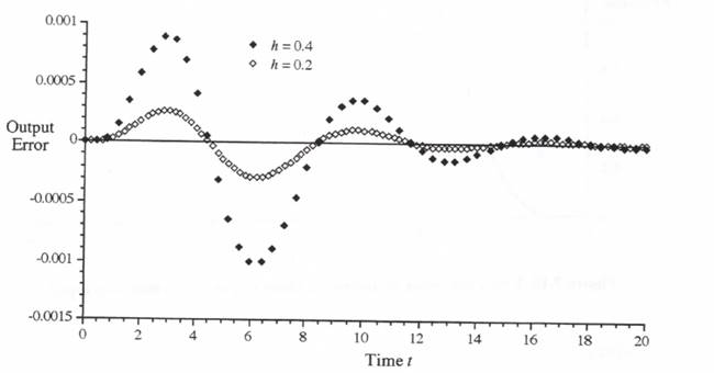
Figure 7.20. Unit step response errors of 6th-order Butterworth filter simulation using modified-Euler simulation with root matching and quadratic compensation.
In the results shown in Figures 7.19 and 7.20 the modified Euler simulation with root matching employed input averaging. When input averaging is not used, the unit step response errors generally become much larger and are dependent on the time at which the unit step is applied. Only for the case where a step input is applied exactly half-way through the k -1 integration frame will the input sample ![]() at the end of the frame equal the average input value over the interval from
at the end of the frame equal the average input value over the interval from ![]() to
to ![]() . The advantage of using modified-Euler integration with input averaging for step-function inputs is discussed further in Chapter 11.
. The advantage of using modified-Euler integration with input averaging for step-function inputs is discussed further in Chapter 11.
The very high accuracy attainable using modified Euler integration with root matching and quadratic compensation suggests that we can consider simulation of the 6th-order Butterworth filter using quite a large step size, accompanied by interpolation to produce an accurate multi-rate output. For example, consider the following formula for quadratic interpolation over the time interval ah using output data points ![]() and
and ![]() :
:
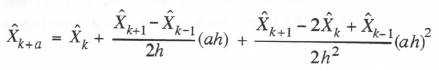
or
(7.106) 
Implementation of Eq. (7.106) requires only two multiplies and two adds per interpolation, since the coefficients for each of the required interpolation intervals can be precomputed. As a specific example, we consider the simulation of the sixth-order Butterworth filter using modified Euler integration with root matching, quadratic compensation, and input averaging when the input is again a unit step at t = 0 . We let the integration step size h = 1 and employ interpolation to produce an output data sequence at five times the integration frame rate. In this case the dimensionless extrapolation interval a in Eq. (7.106) takes on the values 0, 0.2, 0.4, 0.6, and 0.8. The resulting simulation is shown in Figure 7.21. Despite the very large step size ![]() since
since ![]() , the solution, including the multi-rate data sequence obtained by interpolation, is quite close to the result that would be obtained when using an integration step size h = 0.2. The actual error of both the main data sequence output with h = 1 and the interpolated data points is shown in Figure 7.22. The peak error is approximately 1 percent, with the root mean square error much smaller than this.
, the solution, including the multi-rate data sequence obtained by interpolation, is quite close to the result that would be obtained when using an integration step size h = 0.2. The actual error of both the main data sequence output with h = 1 and the interpolated data points is shown in Figure 7.22. The peak error is approximately 1 percent, with the root mean square error much smaller than this.
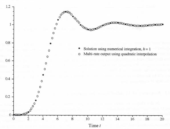
Figure 7.21. Filter step response using modified-Euler integration, root matching and quadratic compensation, h = 1; multi-rate output using quadratic interpolation.
In the interpolation formula of Ect (7.106) it is apparent that the interpolated output over the kth integration frame, ![]() , requires
, requires ![]() , the compensated output at the end of the frame. In a real-time simulation this means that a one-frame lead in the computed output
, the compensated output at the end of the frame. In a real-time simulation this means that a one-frame lead in the computed output ![]() is required. When this is added to the half-frame lead necessary to accommodate input averaging and the one-
is required. When this is added to the half-frame lead necessary to accommodate input averaging and the one-
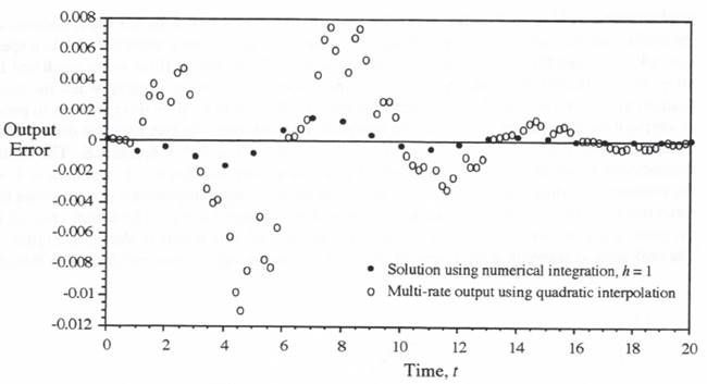
Figure 7.22. Error in multi-rate output illustrated in Figure 7.21.
frame lead required to mechanize the quadratic compensation formula of Eq. (7.105), the total required time advance to produce the real-time multi-rate output becomes two and one-half frames. We have seen that the difference equations represented by (7.101) only provide a two-frame lead. Thus the multi-rate example considered here falls one-half frame short of being able to produce a real-time output. We do note from Eq. (7.101) that an additional one-frame lead can be realized if the order of the Butterworth filter is raised from six to eight. Also, a real-time multi-rate output may not be necessary in many simulations, in which case the method illustrated here can save a great deal of computing time.
7.14 Summary of Modified-Euler Integration Results
In this chapter we have seen how a simple version of modified Euler integration can be used to simulate linear second-order systems. For lightly-damped systems the method is especially effective, and it exhibits exactly zero damping when the system being simulated is undamped. Improvement in both accuracy and stability can be obtained by selecting the coefficients in the difference equation such that the characteristic roots of the digital simulation match exactly those of the continuous system. This is easily accomplished using simple analytic formulas. The resulting algorithm provides better accuracy than any conventional 2nd-order integration method and only requires the same number of adds and multiplies as standard Euler integration.
For the case where velocity rather than displacement represents the output of the second-order system, the modified Euler method yields 2nd-order accuracy if the output velocity is interpreted as occurring at half-integer frame times. The algorithm can be used in simulating any order of linear system, although it is especially straightforward to use in the simulation of higher order systems that consist of second-order linear systems in series. In particular, we have shown how it can be used for very efficient simulation of high-order bandpass and lowpass filters. Modified Euler integration can also be used to simulate nonlinear systems by evaluating each nonlinear state-variable derivative halfway through the integration interval.
Finally, we have shown that it is straightforward to add quadratic compensation to the modified Euler algorithm such that the 2nd-order errors are canceled when simulating a linear system. This results in a 4th-order algorithm with respect to transfer function gain and phase errors. When used to simulate linear filters, the method then exhibits better accuracy than RK-4 integration and executes more than four times as fast.