Simulation of physical systems using digital computers continues to play an ever increasing role in all aspects of today’s technological society. In general the basis for simulation resides in mathematical models of the systems being simulated. In the case of continuous dynamic systems these models consist of either nonlinear ordinary or partial differential equations. The simulation of these systems and hence the simulation of the corresponding mathematical models can be accomplished by numerical integration of the differential equations.
When simulation involves inputs and outputs in the form of real-world signals, either continuous or discrete, it is necessary for the simulation to run in “real time.” In other words, the simulation must be capable of running fast enough on the digital computer that the computed outputs, in response to real-time inputs, occur at the exact time these outputs would take place in the real world. A typical example of this is the real-time flight simulator shown in Figure 1.1. It consists of a digital simulation of the airplane equations of motion interfaced to outputs from and inputs to the actual hardware that will ultimately be used to control the airplane in flight. The system in Figure 1.1 is known as a “hardware-in-the-loop” simulation. It can be used to check out the flight control system under a variety of simulated flight conditions, all in a safe and repeatable laboratory environment. In many cases the “hardware” is a pilot, and the resulting simulation is used to evaluate the flying qualities of the airplane, along with the effectiveness of the cockpit controls and displays. Alternatively, such a man-in-the-loop simulation can be used to train pilots to fly the airplane and handle emergency conditions, again in a safe and controlled environment.
Often the inputs and outputs for a hardware-in-the-loop simulation are in continuous or analog form. In this case the continuous inputs must be converted to digital form using A to D (Analog to Digital) converters, a single channel of which is shown in the figure. The output of the A to D converter is then a data sequence, usually with a fixed time interval h between samples of the analog input. In this case h usually (but not always) becomes the step size for the numerical integration of the airplane equations of motion, as mechanized on the digital computer. The computer outputs, in the form of data sequences, are converted to continuous form using D to A (Digital to Analog) converters, a single channel of which is also illustrated in Figure 1.1. When the hardware is a human operator in a piloted flight simulator, the computer inputs, converted from analog to digital signals, represent the control input displacements generated by the pilot. The computer outputs, converted from digital to analog signals, represent cockpit analog instrument readings, inputs to the motion system (in the case of moving-base simulators), and inputs to any visual display systems.
In addition to continuous inputs and outputs, the hardware in Figure 1.1 may have input/output signals which are digital data sequences, as in the case of a digital flight control system. Also, many of the input/output channels may be simple on-off signals, each of which represents the occurrence of a discrete event.
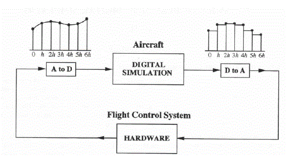
Figure 1.1. Hardware-in-the-loop flight simulation.
There are many other examples of digital simulation involving real-time inputs and outputs, including spacecraft simulators, land vehicle simulators, ship simulators, process control simulators, power plant simulators, etc. As in the flight simulator example of Figure 1.1, the hardware in the loop may be a human operator, in which case the simulator can be used for man-systems development and evaluation, or for the training of human operators.
In real-time digital simulation the numerical integration step size h is almost always fixed. The reason for this is to ensure that the computer will produce outputs at the end of each integration step that never occur later than real time. A fixed step size also ensures compatibility with fixed sample-rate inputs and outputs. The mathematical step size h must of course be chosen large enough that the computer has sufficient available time during each step to finish the necessary calculations. On the other hand, the step size h cannot be made too large, or the errors due to the numerical integration algorithms will cause the dynamic fidelity of the simulation to be unacceptable. Often these dynamic errors (known as integration truncation errors) can be reduced for a given step size h by choosing the proper integration algorithm, by using specialized integration methods, by running fast subsystems with smaller integration steps, and by the use of other special techniques which will be covered in this text.
In order to assess the comparative accuracy of different integration methods and to develop specialized integration algorithms, it is important to have a general method of quantitative evaluation of the dynamic errors in digital simulation. Unfortunately, there is no such method which provides generally useful results when the simulation involves nonlinear differential equations. Fortunately, however, many if not most dynamic systems can be approximated as quasi-linear, time-invarient systems by considering linearized perturbation equations with respect to steady-state or reference solutions over at least limited segments of time. For example, this is precisely the technique used to linearize the highly nonlinear equations of motion of an aircraft in order to develop airframe transfer functions in the design of flight control systems.
When the differential equations are linear and the integration step size is fixed, we can use the method of Z transforms to obtain direct measures of simulation accuracy for specific integration algorithmns.* These direct measures include the fractional error in characteristic roots of the digital simulation, and the fractional error in transfer function gain and the transfer function phase error of the digital simulation. These latter two error measures are particularly useful in determining the acceptability of digital system errors in hardware-in-the-loop simulations, since they can be translated directly into gain and phase-margin errors for the closed-loop simulation.
In this chapter we will introduce a number of conventional integration algorithms which are usually considered in real-time digital simulation. Each of the algorithms will be examined in regard to its suitability for use with real-time inputs. This will be followed by development of the dynamic error measures described above. A brief introduction to Z transforms and their application to digital simulation is presented in Chapter 2. In Chapter 3 we develop both exact and approximate asymptotic formulas for dynamic errors in applying integration algorithms to the simulation of linearized systems. This will allow us to compare the different integration methods and to establish accuracy/speed tradeoffs. Sampling, extrapolation, and interpolation and their application to real-time interface systems is covered in Chapters 4 and 5. Chapter 6 describes and analyzes special methods for simulating linear subsystems, including the state-transition method and Tustin’s method. In Chapter 7 we introduce a modified form of Euler integration which is especially efficient in the simulation of mechanical dynamic systems, where acceleration is integrated to obtain velocity and displacement, respectively. The application of multi-rate integration to the simulation of dynamic systems that can be partitioned into identifiable fast and slow subsystems is described in Chapter 8. Although real-time simulation has traditionally employed fixed integration steps, Chapter 9 shows that variable-step real-time integration can also be utilized and in fact can lead to improved simulation accuracy when computer execution times vary from one integration step to another. To accept real-time inputs and produce real-time outputs, variable-step integration must utilize extrapolation and interpolation. Chapter 10 describes how the variable-step methodology in Chapter 9 can be combined with the multi-rate integration of Chapter 8 to permit real-time asynchronous simulation of complex dynamic systems using either single or multiple processors. Chapter 11 describes methods for handling dynamic systems with discontinuous inputs and discontinuous nonlinearities.
It should again be noted that all of the integration methods considered here in Chapters 1 through 8 use a fixed integration step size because of the real-time requirement. In non real-time simulation this is not necessary, and integration algorithms are often used which vary the step size during the solution based on some error criterion. Even in this case, however, the step size may remain relatively fixed over significant lengths of time, in which case the dynamic analysis techniques developed here can be applied. It may also be true that the use of very efficient fixed-step integration algorithms may actually speed up many non-real-time simulations in comparison with variable-step methods. For a given accuracy, any significant speed improvement will, of course, save computational cost in the non real-time environment.
1.2 Introduction to Numerical Integration Algorithms
In this section we will introduce and interpret a number of integration methods which are candidates for use in real-time digital simulation. We will assume that the continuous dynamic system to be simulated is represented by the following nonlinear differential equation:

(1.1)
Here X is the state vector and U(t) is the input vector. For a qth-order dynamic system with m inputs the scalar equations can be written as

(1.2)
When solving Eq. (1.1) or (1.2) using numerical integration with a fixed integration step size h, we will be computing the vector solution X only at the discrete, equally-spaced time 0, h, 2h, 3h, … . At the time we denote the solution by . Similarly, we denote by . To illustrate the geometric interpretation of numerical integration we consider the simple first-order equation

(1.3)
Given the value of x at t = nh, i.e., given xn, we can express xn+1, i.e., the value of x at t = (n+1)h, by the formula

(1.4)
The integral in Eq. (1.4) is simply the area under the f(t)versus t curve between t = nh and t = (n+1)h, as shown graphically in Figure 1.2. However, in our digital simulation we do not have a representation of the continuous time function f(t). Instead, we have only the representation of f at the discrete times (n-1)h, nh, (n+1)h, … , i.e., fn-1, fn, fn+1, … , Thus we can only approximate
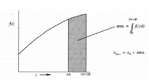
Figure 1.2. Graphical representation of one integration step.
f(t)and hence the area under f(t)using the available values of f at the discrete times. The method used to approximate the area defines the type of numerical integration which will be used.
The simplest integration algorithm is Euler or rectangular integration. In this method the area is approximated by the rectangle of height fn and width h, as shown in Figure 1.3. Thus the area is equal to hfn and the integration formula is given by
![]()
(1.5)
One way of determining the dynamic error associated with Euler integration is to write the Taylor series expansion for x[(n+1)h] about x[nh], i.e.,

(1.6)
From Eqs. (1.5) and (1.6) we can write the following approximate formula for the error in the Euler representation for the area under f(t) versus t over the nth integration frame:

(1.7)
This is known as the local truncation error.* It represents the numerical integration error per integration step. Since there are 1/h steps per unit time, the numerical integration error per unit time is 1/h times the local truncation error, i.e., –hfn′/2 in the Euler integration case considered here. This is known as the global truncation error, which we will denote as eglobal. Clearly the global error associated with Euler integration is proportional to the first power of the integration step size h. For this reason it is denoted as a first-order integration algorithm.
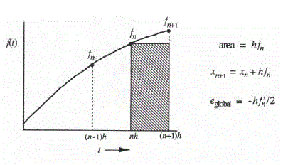
Figure 1.3. Euler integration for the equation dx/dt = f(t)
A more accurate numerical integration formula is obtained by considering the area under the trapezoid shown in Figure 1.4. In this case the algorithm, known as trapezoidal integration, is given by

(1.8)
In this case the local integration truncation error can be derived by considering the Taylor series expansion for fn+1about fn. Thus

from which

(1.9)
Substituting Eq. (1.9) for hfn′ into Eq. (1.6), we obtain the following Taylor series formula for x[(n+1)h]:

(1.10)
Comparison with Eq. (1.8) shows that the local truncation error for trapezoidal integration is given by h3fn″/12. The corresponding global truncation error is then h2fn″/12 . Thus trapezoidal integration is a second-order method, with global errors proportional to h2.
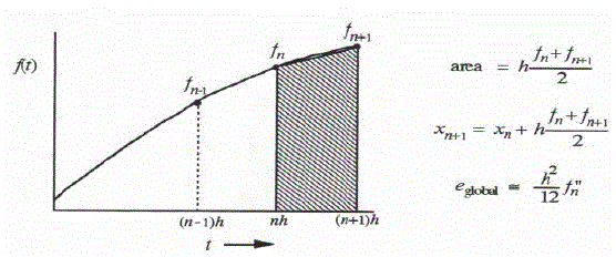
Figure 1.4. Trapezoidal integration for the equation dx/dt = f(t) .
It should be noted that if f in Eq. (1.3) is a function of the state x and an input u(t), i.e., if the first-order equation is given by

(1.11)
then fn+1 in Eq. (1.8) will involve xn+1. If f is a linear function of x, the resulting equation can be solved explicitly for xn+1. In this case the technique is known as Tustin’s method for simulating linear systems. However, if f is a nonlinear function of x, the resulting equation for xn+1 can in general only be solved by some iterative technique. Because of uncertainties in the number of iterations required, especially in dealing with high order systems, implicit trapezoidal integration is generally deemed unsuitable for real-time simulation. It is often used in non real-time simulation, especially in the case of “stiff” systems.* This is because of the robust stability associated with the trapezoidal algorithm. The stability issue will be treated later in Chapters 2 and 3.
The trapezoidal integration formula of Eq. (1.8) also forms the basis for both the Runge-Kutta and Adams-Moulton integration algorithms of second order, as we shall see later in this section.
The difficulties associated with implicit trapezoidal integration when solving nonlinear state equations can be avoided by basing the incremental area under the f(t) versus t curve on a linear extrapolation using fnand fn-1 , as shown in Figure 1.5. The resulting integration algorithm is known as the second-order Adams-Bashforth method, hereafter referred to as AB-2. The integration formula is the following:

(1.12)
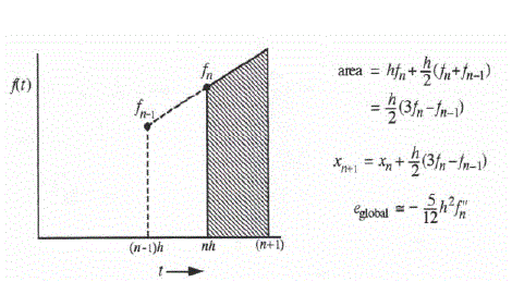
Figure 1.5. AB-2 integration for the equation dx/dt = f(t).
To obtain the formula for the local truncation error we consider the Taylor series expansion for fn-1about fn, from which it is easy to show that

(1.13)
Substituting Eq. (1.13) for hfn′into Eq. (1.6), we obtain the following Taylor series formula for x{(n+1)h]:

(1.14)
Comparison with Eq. (1.12) shows that the local truncation error for AB-2 integration is given by -5h3fn″/12. The corresponding global truncation error is then -5h2fn″/12. Thus AB-2 integration is a second-order method, with global errors proportional to h2.
Implicit third-order integration is illustrated in Figure 1.6. Here a quadratic is passed through the three points fn+1, fn, and fn-1 to approximate f(t) and therefore define the area from t = nh to t = (n+1)h. This leads to the following formula:
![]()
(1.15)
Following the same procedure used for the earlier integration algorithms, it is straightforward to show in this case that the global truncation error is approximately equal to . As in the case of trapezoidal integration, this third-order method involves an implicit equation for xn+1 when f is a nonlinear function of x. This in general will mean iterations to solve for xn+1, which makes the algorithm unsuitable for most real-time simulations.
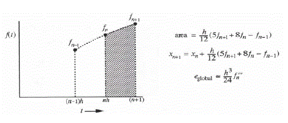
Figure 1.6. Third-order implicit integration for the equation dx/dt = f(t).
A third order explicit integration algorithm can be obtained, however, by passing a quadratic function through the three points fn, fn-1, and fn-2. The area under the resulting curve from t = nh to t = (n+1)h leads the algorithm known as the AB-3 predictor method. From Figure 1.7 we see that the integration formula is
![]()
(1.16)
In this case it can be shown that the global truncation error is equal to -3h2fn‴/8.
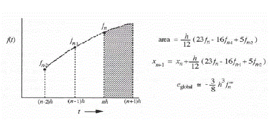
Figure 1.7. AB-3 integration for the equation dx/dt = f(t).
A fourth-order implicit algorithm can be generated by passing a cubic through the four points fn+1, fn, fn-1, and fn-2 to determine the incremental area from t = nh to t = (n+1)h. This leads to the formula
![]()
(1.17)
For this fourth-order implicit integration method it can be shown that the global truncation error is given approximately by 19h4fn(iv)/720.
The explicit AB-4 predictor algorithm is obtained by passing a cubic through the four data points fn, fn-1, fn-2, and fn-3. The resulting cubic extrapolation defines the incremental area from t = nh to t = (n+1)h, which leads to the AB-4 formula
![]()
(1.18)
Here it can be shown that the approximate global truncation error is equal to -251h4fn(iv)/720 .
It should be noted in the AB-2, AB-3, and AB-4 algorithms of Eqs. (1.12), (1.16) and (1.18), as well as in the implicit algorithms of Eqs. (1.15) and (1.17), that in each case the next state X n+1 depends not only on the current state Xnbut also on the past state or states, Xn-1, Xn-2, etc. The presence of these past states in the difference equations means that when using any of these integration algorithms, we are introducing extraneous states not present in the original continuous system being simulated. This in turn tends to reduce the stability of the integration algorithm as the step size h is increased. In Chapter 3 we will examine the stability of these integration methods in detail. The dependence of integration algorithms on past states also causes an initial startup problem, since for n= 0 it implies that X-1, X-2, etc., must be specified as well as X0. One way of solving the startup problem for AB-2 is to use Euler integration for the initial step, followed by AB-2 from then on. In the case of AB-3 we can use Euler for the first step, AB-2 for the second, and AB-3 from then on. For AB-4 we start with Euler, then AB-2, AB-3, AB-4, AB-4, AB-4, etc. A similar approach can be used to solve the startup problem for the implicit algorithms. For example, the third-order implicit method can be started using the trapezoidal integration of Eq. (1.8) for the first step, followed by the third-order implicit integration of Eq. (1.15) for all subsequent steps.
The third-order Formulas in Eqs. (1.15) and (1.16) form the basis for the third-order Adams-Moulton predictor-corrector integration algorithm, hereafter referred to as AM-3 integration. In the same way, Eqs. (1.17) and (1.18) form the basis for the AM-4 predictor-corrector algorithm. In considering the explicit Adams-Moulton methods in general, we will write the formulas for the numerical integration of the vector state equation as given in (1.1). In the case of AM-2 integration, a predicted value, n+1, for the next state is computed using the AB-2 formula of Eq. (1.12). n+1 is then used instead of Xn+1, to calculate the derivative Fn+1 in the trapezoidal formula of Eq. (1.8). Thus the AM-2 algorithm is given by
![]()
(1.19)
![]()
(1.20)
The AM algorithms are called predictor-corrector methods, where the calculation of n+1 using the AB algorithm is viewed as the predictor, and the calculation of Xn+1 using the implicit algorithm is viewed as the corrector. We have already seen that the local truncation error associated with n+1 in Eq. (1.19) is proportional to h3. Thus the global truncation error of order h2 associated with the trapezoidal algorithm of Eq. (1.20) is not affected by the error of order h3 associated with the use of n+1 instead of Xn+1 in mechanizing Eq. (1.20). This in turn means that the approximate global truncation error of the two-pass AM-2 algorithm is the same as the global error associated with true implicit trapezoidal integration, namely h2fn″/12 as noted earlier in Figure 1.4.
In the case of AM-3 integration, a predicted value, n+1 , for the next state is computed using the AB-3 formula of Eq. (1.16). n+1 is then used instead of Xn+1, to calculate the derivative Fn+1 in the third-order implicit formula of Eq. (1.15). Thus the AM-3 algorithm is given by
![]()
(1.21)
![]()
(1.22)
For the reasons cited above for AM-2, the approximate global truncation error of the two-pass AM-3 algorithm is the same as the global error associated with true implicit third-order integration, namely h2fn‴/24, as noted earlier in Figure 1.6.
For AM-4 integration a predicted value, n+1 for the next state is computed using the AB-4 formula of Eq. (1.18). n+1is then used instead of Xn+1, to calculate the derivative Fn+1 in the fourth-order implicit formula of Eq. (1.17). Thus the AM-4 algorithm is given by
![]()
(1.23)
![]()
(1.24)
Again, for the reasons cited above for AM-2, the approximate global truncation error of the two-pass AM-4 algorithm is the same as the global error associated with true implicit fourth-order integration, namely 19h2fn(iv)//720 as noted earlier following Eq. (1.17).
The Adams-Moulton predictor-corrector algorithms combine the accuracy of the implicit methods with the explicit nature of the AB predictor methods. We now turn to the consideration of some Runge-Kutta integration algorithms. First we introduce a second-order Runge-Kutta (RK-2) method also known as Heun’s method. As in the case of AM-2, we first compute an estimate, n+1 for the next state. But in RK-2 integration, this estimate is computed using Euler integration n+1. is then used to calculate the derivative Fn+1 in the trapezoidal formula of Eq. (1.8). The algorithm is therefore given by the following two equations:
![]()
(1.25)
![]()
(1.26)
An interesting variation of the above RK-2 method uses Euler integration in the first pass to compute n+1/2, an estimate of the state halfway through the next integration step. n+1/2 is then used to compute the derivative Fn+1/2 at the half-integer step which, in turn, is used to compute Xn+1 The two equations for the algorithm are
![]()
(1.27)
![]()
(1.28)
One advantage of this second RK-2 method is its compatibility with real-time inputs. Since both RK-2 methods above are two pass algorithms, i.e., they each require two evaluations of the state-variable derivative F per integration step, it is reasonable to assume that each pass will require approximately the same time to execute on a given computer. At the beginning of the first pass, that is, at t = nh, the input Un has just become available in real time. However, at the beginning of the second pass, at t = h/2, the RK-2 formula in Eq. (1.26) requires Un+ 1 , i.e., the input at t = (n+1)h, which is not yet available in real time. However, the RK-2 formula in Eq. (1.28) only requires Un+1/2 at the beginning of the second pass, which is available in real time. For this reason the second algorithm is denoted as RTRK-2, to indicate its compatibility with real-time inputs. In Chapter 3 we will examine in some detail the dynamic errors associated with both the RK-2 and RTRK-2 algorithms. In each case the global truncation errors are proportional to h2.
Reference to the AB-2, AB-3, and AB-4 algorithms presented earlier in Eqs. (1.12), (1.16) and (1.18) shows that they are all single-pass methods, that is, they require only one evaluation of the state-variable derivative per integration step. Since at the beginning of the step, i.e., at t = nh, the required input Un at t = nh is available in real time, the AB methods are compatible with real-time inputs. On the other hand, the implicit algorithms in Eqs. (1.8), (1.15) and (1.17), as well as the second pass in Eqs. (1.20), (1.22) and (1.24) for the two-pass AM algorithms, all require Un+1, i.e., the input at t = (n+1)h, which in each case is not yet available in real time. Thus none of the implicit or AM methods presented thus far are compatible with real-time inputs. Of course one can employ extrapolation, for example based on Un and past input samples, to compute an estimate ûn+1 for use instead of Un+1 in the formulas, but this introduces significant additional dynamic errors, as we shall see in Chapter 4.
There is, however, a way to construct a family of two-pass AM predictor corrector algorithms which are compatible with real-time inputs. The second-order member of this family is based on using a second-order predictor method instead of Euler integration to compute the state estimate n+1/2, halfway through the frame. This is then followed by the modified Euler equation given in (1.28) for the second pass. Thus the equations become the following:
![]()
(1.29)
![]()
(1.30)
Because the predictor corrector algorithm given by Eqs. (1.29) and (1.30) is compatible with real-time inputs, i.e., Un+1/2 is required at the start of the second pass for Eq. (1.30), just when it becomes available in real time, we designate the method as RTAM-2. To determine the formula for the predictor pass in the RTAM-2 algorithm we represent F(t) with a linear approximation which passes through Fn and Fn-1. The incremental area in the predictor formula is then based on the integral of the linear F(t) approximation from t = nh to t = (n+1/2)h, namely, h(5Fn – Fn-1)/8 on the right side of Eq. (1.29). It can be shown that the global truncation error for RTAM-2 is given approximately by –h2Fn″/24.
For RTAM-3 the predictor estimate, n+1/2 is based on the area from t = nh to t = (n+1/2)h under a quadratic approximation for F(t) which passes through Fn, Fn-1 and Fn-2. This is followed by the corrector formula for Xn+1, which is based on the area from t = nh to t = (n+1)h under a quadratic approximation for F(t) which passes through Fn+1/2, Fn and Fn-1, where Fn+1/2 has been evaluated using n+1/2 and Un+1/2. This leads to the following two equations:
![]()
(1.31)
![]()
(1.32)
It is straightforward to show that the global truncation error for RTAM-2 is given approximately by –h3Fn‴/36.
For RTAM-4 the predictor estimate, n+1/2 is based on the area from t = nh to t = (n+1/2)h under a cubic approximation for F(t) which passes through Fn, Fn-1, Fn-2 and Fn-3. This is followed by the corrector formula for Xn+1, which is based on the area from t = nh to t = (n+1)h under a cubic approximation for F(t) which passes through Fn+1/2, Fn, Fn-1 and Fn-2, where Fn+1/2 has been evaluated using n+1/2 and Un+1/2. This leads to the following two equations:
![]()
(1.33)
![]()
(1.34)
The global truncation error for RTAM-4 turns out to be equal approximately to -59h4Fn(iv)/2880.
Having developed the real-time AM predictor-corrector formulas by analogy with the RTRK-2 method, let us return to a consideration of higher-order Runge-Kutta methods. One version of RK-3 integration uses the following equations:
![]()
(1.35)
![]()
(1.36)
![]()
(1.37)
Here Euler integration with a step size equal to h/3 is used in Eq. (1.35) to compute n+1/3 which, in turn, is used to compute Fn+1/3. Euler integration with a step size equal to 2h/3 then uses Fn+1/3 in Eq. (1.36) to compute, n+2/3 from which Fn+2/3 is computed. Finally, Fn and Fn+2/3 are used in Eq. (1.37) to compute Xn+1. Comparison of Eqs. (1.35) and (1.36) with Eqs. (1.27) and (1.28) for RTRK-2 shows that they are identical if one replaces h in Eqs. (1.27) and (1.28) with 2h/3 in Eqs. (1.35) and (1.36). It follows that n+2/3 in Eq. (1.37) is generated using RTRK-2 integration with a step size of 2h/3 instead of h.
In Chapter 3 we will examine in detail the dynamic errors associated with the RK-3 algorithm introduced here, as well as show that the global dynamic errors are proportional to h3. We note that RK-3 is a three-pass algorithm, since it requires three evaluations of the state-variable derivative per integration step. It is reasonable to assume that each pass will take approximately the same time to execute on a given computer, that is, each pass will take approximately h/3 seconds. When the first pass is initiated at t = nh, Eq. (1.35) requires the input Un, which has just become available in real time. At the beginning of the second pass, t = h/3 and Eq. (1.36) requires Un+1/3 which once more has just become available in real time. At t = 2h/3 the third and final pass begins and Eq. (1.37) requires the input Un+2/3 which, again, has just become available in real time. Thus the above RK-3 algorithm is compatible with real-time inputs, since in a real-time simulation the algorithm never requires inputs before they occur in real time.
The final integration algorithm considered is RK-4, a fourth-order Runge-Kutta method which has been very widely used for numerical integration. The RK-4 equations are summarized below:
![]()
(1.38)
![]()
(1.39)
![]()
(1.40)
![]()
(1.41)
Since the RK-4 algorithm shown here requires four derivative evaluations, each total integration step will require four passes through a state equation to evaluate the necessary derivatives F. It follows that each pass will take h/4 seconds. Thus at the beginning of the second pass, at which time t = h/4, Eq. (1.39) requires Un+ 1/2, which is h/4 seconds ahead of when it becomes available in real time. Similarly, at the beginning of the fourth pass, at which time t = 3h/4, Eq. (1.41) requires Un+1, which again is h/4 seconds ahead of when it becomes available in real time. We therefore conclude that RK-4 is not an algorithm compatible real-time inputs. In Chapter 3 we will examine in detail the dynamic errors associated with the RK-4 algorithm defined here, as well as show that the global dynamic errors are proportional to h4.
1.3 Dynamic Error Measures
The final topic considered in this introductory chapter is the error measures which we will use to compare different integration methods in the simulation of dynamic systems. As noted earlier, we will assume that we can linearize the nonlinear state equations about some reference or equilibrium solution. Then the dynamic relationship between any scalar input-output pair can be represented in terms of a transfer function given by

(1.42)
Here we have assumed a linearized system of order q with characteristic roots (i.e., transfer function poles) given by, λ1, λ2, …, λqThus the system being simulated is of qth order. If there are no repeated roots, H(s) in Eq. (1.42) can be represented in terms of the following partial fraction expansion:

(1.43)
where

(1.44)
For the case where λk and λk+1 represent a complex-conjugate pair, the two resulting first-order transfer functions with complex conjugate coefficients Ak and Ak-1 can be combined into a second-order transfer function with real coefficients. Thus a qth-order linear system with distinct roots can be represented as the sum of first and second-order linear subsystems. If we can determine the dynamic errors in simulating these subsystems, then by superposition we can determine the overall dynamic error in solving the quasi-linear version of the entire system being simulated. This in turn can give us insight into the dynamic errors when simulating the full nonlinear system.
We shall use two types of error measures in our analysis. The first is eλ, the fractional error in characteristic root, defined as

(1.45)
Here λ* is the equivalent characteristic root in the digital solution, whereas λ is the exact continuous-system root. In Chapter 2 we will see how we can determine λ* using the method of Ztransforms. For the case where λ is complex the resulting complex-conjugate root pair can be expressed in terms of the undamped natural frequency ωn and damping ratio ζ of the corresponding undamped second-order subsystem. Thus we can write
![]()
(1.46)
In this case it is useful to define the fractional error in damped frequency, eω , and the damping-ratio error, eζin accordance with the following formulas:

(1.47)
Here ωd and ωd* represent the damped frequencies, respectively, associated with the continuous system and digital system roots, and are given by
![]()
(1.48)
An alternative measure of complex root frequency error is eωn, the fractional error in complex root undamped natural frequency, defined as

(1.49)
Eq. (1.49) reminds us that the magnitude |λ| of a complex root is in fact its undamped natural frequency ωn. This follows directly by writing the formula for the magnitude of the right hand side of Eq. (1.46). The fractional root error, eλ, as defined earlier in Eq. (1.45), applies equally well to either complex or real roots. Thus eλ will in general have both a real and an imaginary part. In order to have a single error measure in the case of complex roots, it is useful to define e|λ|, the normalized magnitude of the characteristic root error. Thus we let

(1.50)
The various error measures defined above all are concerned with errors of the equivalent characteristic roots in the digital simulation of first or second-order linear subsystems. However, since Eq. (1.43) shows that any linearized system with distinct roots can be represented as the sum of first order (or in the case of complex roots, second-order) subsystems, clearly the above error measures can be used for any order of linearized system. Errors in the equivalent characteristic roots of a digital simulation will of course be directly related to time domain errors in the transient solution.
Until now we have not considered the case of repeated characteristic roots. If the linearized system has m equal real roots, the corresponding subsystem in the partial fraction expansion must be of order m. By considering second-order as well as first-order subsystems, we have already taken care of the case where m = 2. Non-zero repeated roots for m > 2 occur rather infrequently and can be analyzed separately. For m repeated roots equal to zero, the linear subsystem has a transfer function given by 1/sm, for which numerical integration algorithms of the type considered in these notes will not introduce characteristic root errors.
To determine errors associated with the dynamic response of linearized systems to input functions, we turn to frequency-domain considerations. In particular, we choose as an error measure the fractional error in the transfer function of the digital system when the input is a sinusoid of frequency ω. This can be determined from the Z transform, H*(z), of the digital system represented by the computer simulation. In Chapter 2 we will show that for sinusoidal input data sequences, the digital-system transfer function is simply H*(ejωh). Then the fractional error in digital-system transfer function can be written as

(1.51)
Here H(jω) is the transfer function for sinusoidal inputs of the continuous linear system being simulated, and eM and eA represent, respectively, the real and imaginary parts of the fractional error in the transfer function of the digital system. For transfer function error magnitudes small compared with unity, eMand eA have an especially significant meaning, which can be understood by writing H*and H in polar form. Thus we let H* = |H*|ejN* and H=|H|ejN, where |H*| and N* are the gain and phase, respectively, of the digital system, and |H| and N are the gain and phase, respectively, of the continuous system. After substitution into Eq. (1.51), we obtain

(1.52)
Here we have used a first-order power series approximation for ej(N*-N) and neglected terms higher than first order in (N*-N). Also, (|H*|/|H|)-j(N*-N) has been approximated by j(N*-N), since by assumption H* H if the simulation is of reasonable accuracy. Comparison of Eqs. (1.52) and (1.51) shows that

(1.53)

(1.54)
We conclude that the real part, eM , of the fractional error in transfer function corresponds to the fractional error in digital transfer function gain, and the imaginary part, eA, corresponds approximately to the phase error of the digital transfer function.
Another error measure for the digital-system transfer function is eH, the fractional error in transfer function magnitude. Thus

(1.55)
It is straightforward to show that the fractional peak error in sinusoidal output of the digital system is equal to eH. By fractional peak error we mean the peak error over each cycle divided by the peak output amplitude.
As noted earlier, errors in characteristic roots, as reflected by Eqs. (1.45), (1.47), (1.49) or (1.50), will determine how well the transients generated in the digital simulation will match the transients in the continuous system. The fractional error in digital-system transfer function for sinusoidal inputs can be related directly to the overall dynamic error which will be present in a hardware-in-the-loop simulation. Consider, for example, the hardware-in-the-loop simulation shown in Figure 1.1 at the beginning of this chapter. If we break the loop, as shown in Figure 1.8, and let Xin and Xout respectively, be the input and output for the resulting open-loop system, then the open-loop transfer function H0(s), also known as the return ratio, is defined as

(1.56)
It follows that the open-loop transfer function for sinusoidal inputs is simply H0(jω). We recall from traditional control systems theory that the crossover frequency ω0 of a closed loop system is defined as the frequency of unity open-loop gain. Thus by definition
![]()
(1.57)
We also recall that the phase margin of the closed-loop system is the amount by which the open-loop phase shift at the crossover frequency ω0 exceeds -π radians (i.e., -180 degrees). Thus
![]()
(1.58)
If the phase margin is zero, the closed-loop system is neutrally stable at a frequency equal to ω0, the crossover frequency. For the closed loop system to be stable, the phase margin must be positive. The size of the phase margin is a direct measure of the relative stability of the closed-loop system. Typically, a phase margin of the order of π/4 radians (45 degrees) will result in a fairly well-damped closed-loop transient behavior. Also, the crossover frequency itself will be roughly equal to the dominant frequency in the closed-loop transient. Thus the phase margin and crossover frequency are measures of the relative stability and dominant transient frequency of the closed-loop system.
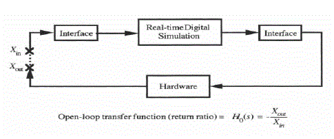
Figure 1.8. Hardware-in-the-loop simulation with feedback loop broken.
For a hardware-in-the-loop simulation to exhibit relative stability which closely matches that of the system being simulated, it follows that the phase error in the digital system transfer function at the crossover frequency ω0 must be sufficiently small. Since ω0 is defined as the frequency of unity open-loop gain, any gain error in the digital-system transfer function will affect the crossover frequency. Thus for a hardware-in-the-loop simulation to exhibit a crossover frequency which closely matches that of the system being simulated, the gain error in the digital-system transfer function at ω0 must also be sufficiently small. Since the dominant frequency in the closed-loop transient will be approximately equal to ω0, small gain error in the digital simulation at that frequency will ensure an accurate representation of the closed-loop transient frequency, just as small phase error at ω0 ensures an accurate representation of the damping for closed-loop transients.
For the above reasons we conclude that transfer function errors in real-time simulation may in general be more important than characteristic root errors, although in Chapter 3 we will develop formulas for both error measures using the method of Z transforms.
